machine learning for chaos system-应用

前言：

前几天，我的导师发给我一个机器学习的案例，说很感兴趣，可不可能应用在我们的实验台上。我当时的回答是我不敢轻易尝试。从做科研的角度，一直觉得这门学科是非线性动力学和统计学的高深理论，十分敬畏。简简单单地拿tensorflow建个模型，算一下，说自己结果可行，那到底思考在哪里呢？对此，我十分怀疑。

但当我开始学习chaos的一些理论，我又不得不开始思考，中间的一些联系。在此，有必要开辟一个章节，学习和感悟这一话题。尽管题目定的很大—机器学习，但着眼的例子很小（例如一维K-S 模型，离散涡模型）。从非线性流体力学系统出发，希望有所感悟。

学习目标：

• 如何构建神经网络模型，来近似模型chaos系统
• 是否chaos系统可以通过AI模型被预测？比如一些critical pattern？
• 如何将AI模型与系统的稳定性相互关联？
• chaos理论的一些思考和机器学习的一些共性？

Challenges and Opportunities for Machine Learning in Fluid Dynamics⁵

Fluid dynamics presents challenges that differ from those tackled in many applications of machine learning, such as image recognition and advertising. In fluid flows it is often important to precisely quantify the underlying physical mechanisms in order to analyze them. Furthermore, fluids flows entail complex, multi-scale phenomena whose understanding and control remain to a large extent unresolved. Unsteady flow fields require algorithms capable of addressing nonlinearities and multiple spatiotemporal scales that may not be present in popular machine learning algorithms. In addition, many prominent applications of machine learning, such as playing video games, rely on inexpensive system evaluations and an exhaustive categorization of the process that must be learned. This is not the case in fluids, where experiments may be difficult to repeat or automate and where simulations may require large-scale supercomputers operating for extended periods of time.

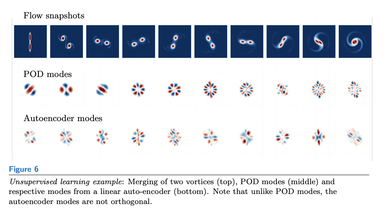
Dimensionality reduction : POD, PCA and auto-encoders

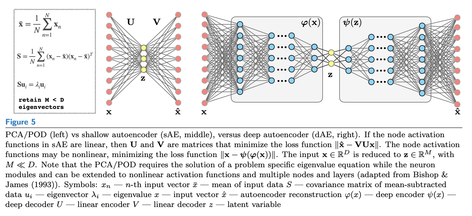
特点：网络两边是对称的

Autoencoder: A neural network architecture used to compress and decompress high-dimensional data. They are powerful alternatives to the Proper Orthogonal Decomposition (POD).

用途：

• 重构流场https://github.com/harsha070/Reconstruction-of-Flows

PDE学习¹⁰

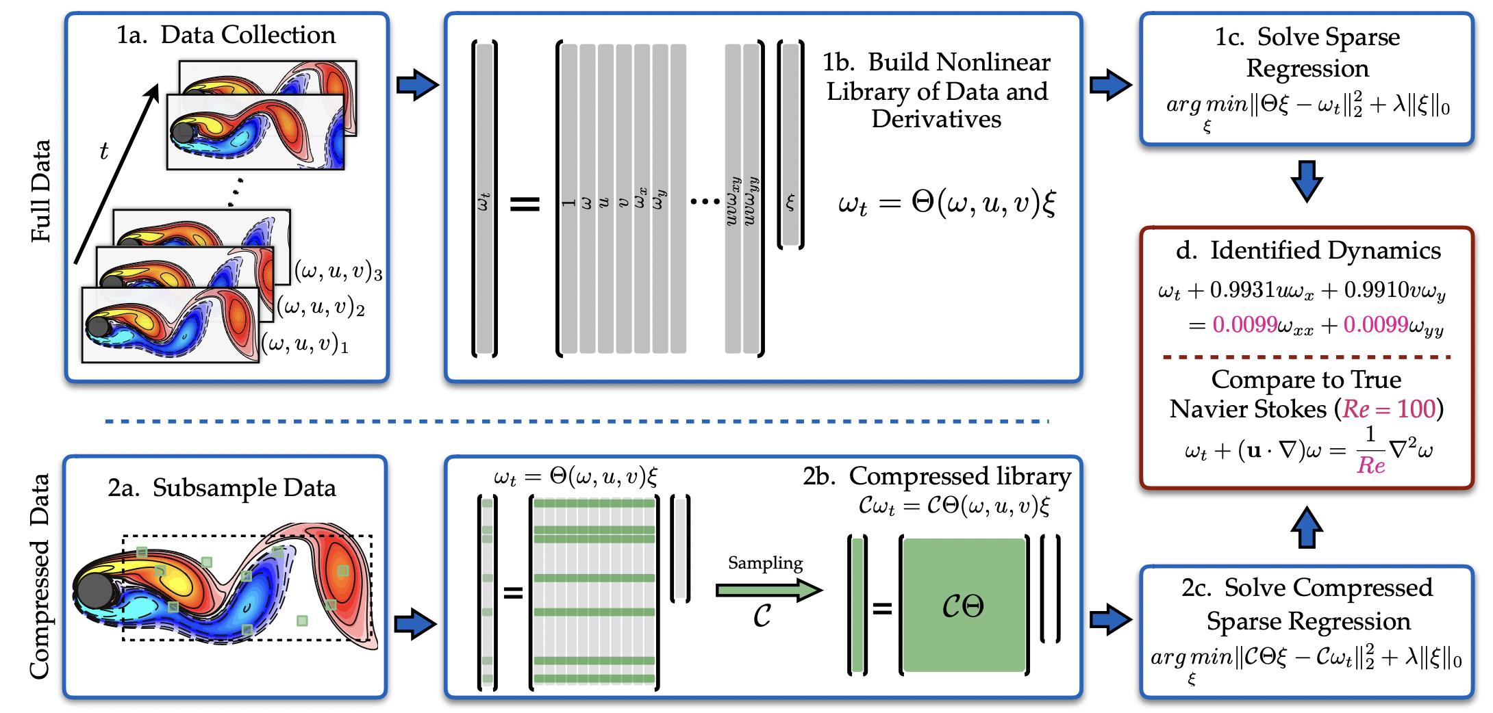
PDE可以统一写成：

$$u_t = N(u,u_x,u_{xx},...,x,t,\mu)$$

其中，$\mu$为系统的参数。Q as a matrix containing additional information that may be relevant, such as dependencies on the absolute value of |u|, or another time varying function inetracting with u.

选择sparse active terms 构建$\Theta$矩阵：

$$\Theta(U,Q)=[1 \space U \space U^2 .. Q..U_x\space UU_x ..Q^2U^3U_{xxx}]$$

行：所有的采样点，列：candidate terms, 各自function计算；

$\xi$便是所要求的系数。

也就是说，，每个点都满足上述方程，无非是求解方程，求出系数。

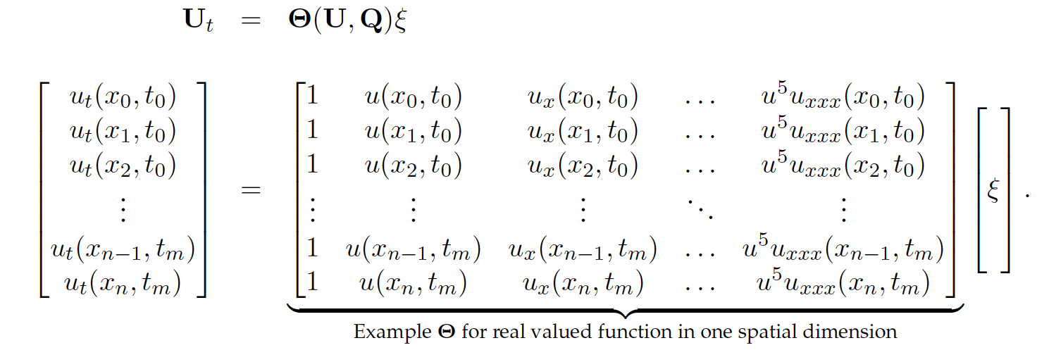
$\Theta$矩阵难免包含数值和测量误差，这里采用sparse regression来求解：

$$\xi = arg \space min_{\hat{\xi}}\left\Vert \Theta \hat{\xi} -\hat{U}_t\right\Vert_2^2 + \lambda \left\Vert \hat{\xi}\right\Vert_0$$

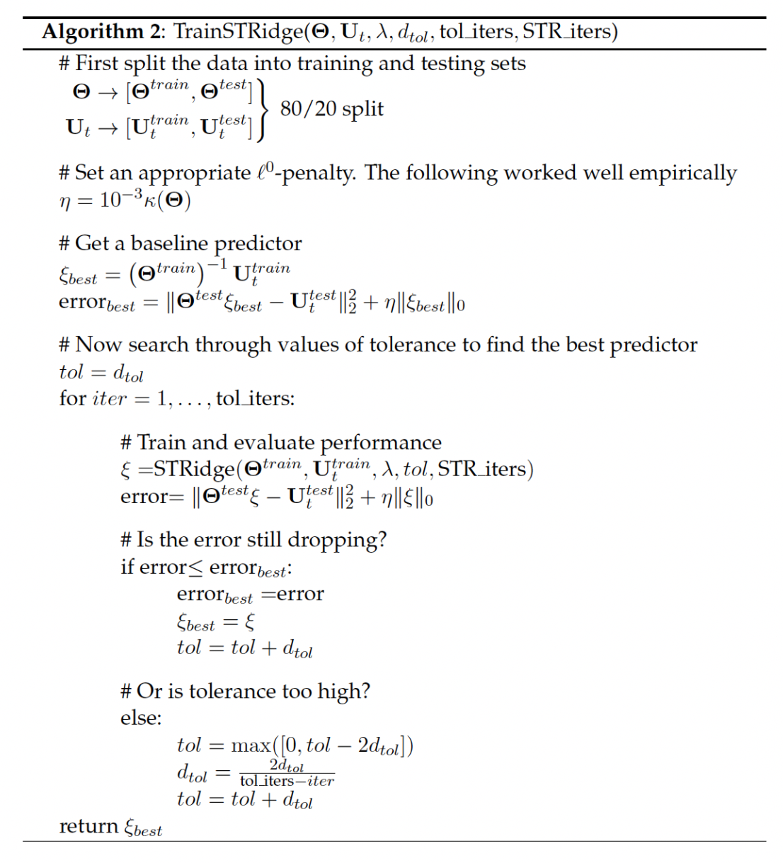
$l_0$ 问题为n-p hard，通过convex relaxation 为$l_1$, 或者 sequentially thresholded least squares(STLS) 为 $l_2$:

$$\xi = arg \space min_{\hat{\xi}}\left\Vert \Theta \hat{\xi} -\hat{U}_t\right\Vert_2^2 + \lambda \left\Vert \hat{\xi}\right\Vert_2\\\\ = (\Theta^T \Theta +\lambda I)^{-1} \Theta^T U_t$$

Numerical Differentition

Use a Gaussian smoothing kernel on noisy data prior to taking derivatives with finite differences. Convolve with a Gaussian.

Tikhonov differentiation finds a numerical derivative $\hat{f}’$ by balancing the closeness of the integral of $\hat{f}’$ to f with the smoothness of $\hat{f}’$.

$$\hat{f}'(x) = arg \space min_g \left\Vert \int_{x0}^x g(s ds -(f(x)- f(x0)))\right\Vert_2^2 + \lambda \left\Vert {dg\over dx} \right\Vert_2^2$$

In the discrete problem, A is a trapezoidal approximation to the integral and D is a finite approximation to the derivative. The problem has closed form solution given by,

$$\hat{f}'= (A^T A + \lambda D^T D)^{-1} A^T f$$

问题：边界附近的differentiate求解误差很大。

闲话：这个算法是否可以应用到管道声学的逆推呀？

PDE-FIND for Burger’s Equation

Samuel Rudy, 2016

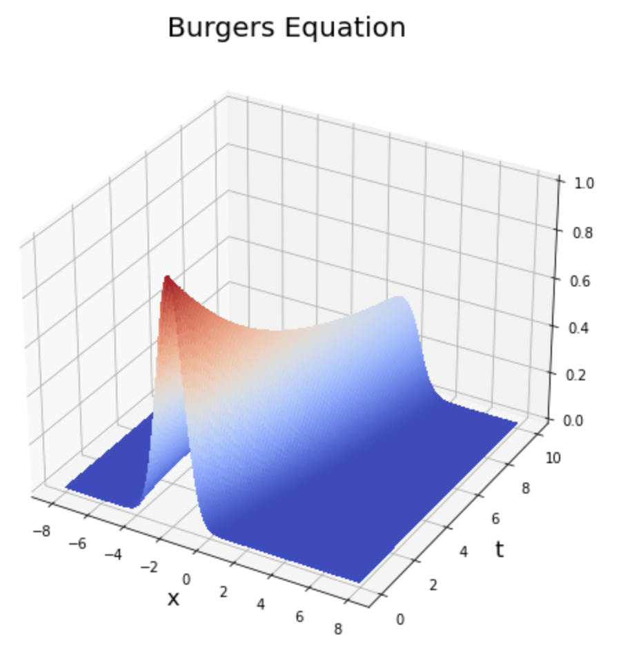
This notebook demonstrates PDE-FIND on Burger’s equation with an added diffusive term.

$$u_t + uu_x = u_{xx}$$

The solution given is a single travelling wave, starting out as a Gaussian.

%pylab inline
pylab.rcParams['figure.figsize'] = (12, 8)
import numpy as np
from mpl_toolkits.mplot3d import Axes3D
sys.path.append('../')
from PDE_FIND import *
import scipy.io as sio
import itertools

Populating the interactive namespace from numpy and matplotlib

data = sio.loadmat('burgers.mat')
u = real(data['usol'])
x = real(data['x'][0])
t = real(data['t'][:,0])
dt = t[1]-t[0]
dx = x[2]-x[1]

print(f'{u.shape}')
print(f'{x.shape}')
print(f'{t.shape}')

(256, 101)
(256,)
(101,)

X, T = np.meshgrid(x, t)
fig1 = figure()
ax = fig1.gca(projection='3d')
surf = ax.plot_surface(X, T, u.T, rstride=1, cstride=1, cmap=cm.coolwarm,
    linewidth=0, antialiased=False)
title('Burgers Equation', fontsize = 20)
xlabel('x', fontsize = 16)
ylabel('t', fontsize = 16)

Text(0.5, 0, 't')

Construct $\Theta (U)$ and compute $U_t$

The function build_linear_system does this for us. We specify

D = highest derivative to appear in $\Theta$

P = highest degree polynomial of $u$ to appear in $\Theta$ (not including multiplication by a derivative.

time_diff and space_diff taken via finite differences

Printed out is a list of candidate functions for the PDE. Each is a column of $\Theta (U)$

Ut, R, rhs_des = build_linear_system(u, dt, dx, D=3, P=3, time_diff = 'FD', space_diff = 'FD')
['1'] + rhs_des[1:]

['1',
 'u',
 'u^2',
 'u^3',
 'u_{x}',
 'uu_{x}',
 'u^2u_{x}',
 'u^3u_{x}',
 'u_{xx}',
 'uu_{xx}',
 'u^2u_{xx}',
 'u^3u_{xx}',
 'u_{xxx}',
 'uu_{xxx}',
 'u^2u_{xxx}',
 'u^3u_{xxx}']

Solve for $\xi$

TrainSTRidge splits the data up into 80% for training and 20% for validation. It searches over various tolerances in the STRidge algorithm and finds the one with the best performance on the validation set, including an $\ell^0$ penalty for $\xi$ in the loss function.

# Solve with STRidge
w = TrainSTRidge(R,Ut,10**-5,1)
print("PDE derived using STRidge")
print_pde(w, rhs_des)

PDE derived using STRidge
u_t = (-1.000987 +0.000000i)uu_{x}
    + (0.100220 +0.000000i)u_{xx}

err = abs(np.array([(1 -  1.000987)*100, (.1 - 0.100220)*100/0.1]))
print("Error using PDE-FIND to identify Burger's equation:\n")
print("Mean parameter error:", mean(err), '%')
print("Standard deviation of parameter error:", std(err), '%')

Error using PDE-FIND to identify Burger's equation:

Mean parameter error: 0.15935000000000255 %
Standard deviation of parameter error: 0.06064999999999543 %

Now identify the same dynamics but with added noise.

The only difference from above is that finite differences work poorly for noisy data so here we use polynomial interpolation. With deg_x or deg_t and width_x or width_t we specify the degree number of points used to fit the polynomials used for differentiating x or t. Unfortunately, the result can be sensitive to these.

numpy.random.seed(0)
un = u + 0.01*std(u)*np.random.randn(u.shape[0],u.shape[1])

Utn, Rn, rhs_des = build_linear_system(un, dt, dx, D=3, P=3, time_diff = 'poly',
                                       deg_x = 4, deg_t = 4, 
                                       width_x = 10, width_t = 10)

# Solve with STRidge
w = TrainSTRidge(Rn,Utn,10**-5,1)
print("PDE derived using STRidge")
print_pde(w, rhs_des)

PDE derived using STRidge
u_t = (-1.009655 +0.000000i)uu_{x}
    + (0.102966 +0.000000i)u_{xx}

err = abs(np.array([(1 -  1.009655)*100, (.1 - 0.102966)*100/0.1]))
print("Error using PDE-FIND to identify Burger's equation with added noise:\n")
print("Mean parameter error:", mean(err), '%')
print("Standard deviation of parameter error:", std(err), '%')

Error using PDE-FIND to identify Burger's equation with added noise:

Mean parameter error: 1.9657499999999966 %
Standard deviation of parameter error: 1.0002499999999996 %

闲话：可以利用上述代码计算单个点的偏导数，这个完全可以直接拿来用。

然后用来计算其他参数，比如刻画涡结构等。。所以，最好还是先用圆柱扰流先做测试。

ML-embedded Universal Differential Equations¹¹

blog：http://www.stochasticlifestyle.com/

https://github.com/ChrisRackauckas/universal_differential_equations

Neural ODE:

$$u' = NN_\theta(u,t)\\\\ NN_\theta(u,t)= W_3\sigma_2(W_2\sigma_1(W_1[u;t]+b_1)+b_2)+b_3\\\\ \theta = (W_1, W_2, W_3, b_1, b_2, b_3)$$

The Universal Approximation Theorem (UAT) demonstrates that sufficiently large neural networks can approximate any nonlinear function with a finite set of parameters.

Universe ordinary differential equation (UODE):

$$u'=f(u,t,U_\theta(u,t))$$

a known mechanistic model form f with missing terms defined by some universal approximation(UA) $U_\theta$.

训练

the cost function $C(\theta)$ by Euclidean distance:

$$C(\theta) = \sum_i \left\Vert u_\theta(t_i)-d_i \right\Vert$$ $${ dC\over d\theta } ->{du\over d\theta}$$

对于一个函数来说，$f(x)=A$

$$x = B_f^x(A)$$

输入x，经过多次f后输出$x_i$:

$$x_i = (f^i \odot f^{i-1} \odot ...\odot f^1)(x)$$

那么，一步一步回撤一段时间L，等价于

$$B_f^x(A) = (B_{f^1}^x (...(B_{f^{L-1}}^{x_{L-2}}(B_{f^L}^{x_{L-1}}(A)))$$

后扯过程可以靠算法实现。例如Zygote.jl

Automated Identification of Nonlinear Interactions

Extend SInDy algorithm(类似time-delay DMD with sparse)， the idea is to find a sparse basis over a given candidate library minimizing the objective function using data.¹¹

UDE approach to extend SinDy that embeds prior structural knowledge.

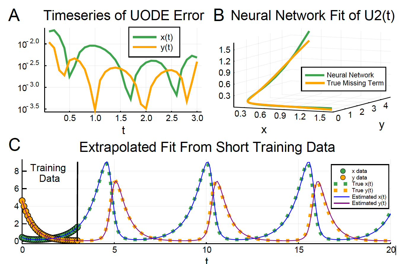
Take Lots-Volterra system as example:

$$\dot{x} = \alpha x - \beta xy\\\\ \dot{y} = \gamma xy -\delta y$$

在只知道部分参数，例如$\alpha,\delta$，可以构建如下knowledge-based UODE:

$$\dot{x}=\alpha x + U_1(x,y),\\\\ \dot{y}=-\delta y+U_2(x,y)$$

可以看到非线性部分，通过$U_1$和$U_2$来模拟。

a system of ordinary differential equations that incorporates the known structure but leaves room for learning unknown interactions between the the predator and prey populations.

问题：是否可以利用这个原理，训练压气机仿真压力和速度之间的关系，从而应用到实验中。伯努利方程为基础。

代码：

卷积与PDE之间的关系

$$\triangle u=u_{xx}+u_{yy}=\\\\ {u(x+\triangle x,y)-2u(x,y)+u(x-\triangle x,y)\over \triangle x^2} + {u(x x,y+\triangle y)-2u(x,y)+u(x,y-\triangle y)\over \triangle y^2} \\\\ +O(\triangle x^2)+O(\triangle y^2)$$

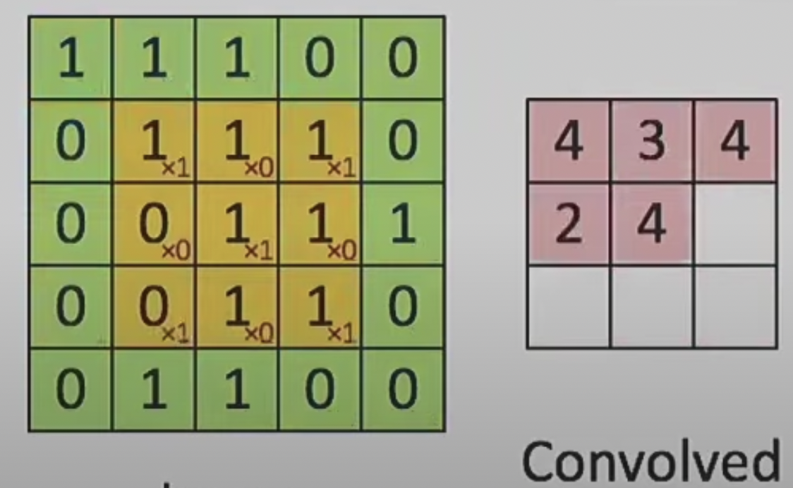
该公式等价于卷积核为：

0	1	0
1	-4	1
0	1	0

Neural PDE 加速仿真计算

MIT-climate

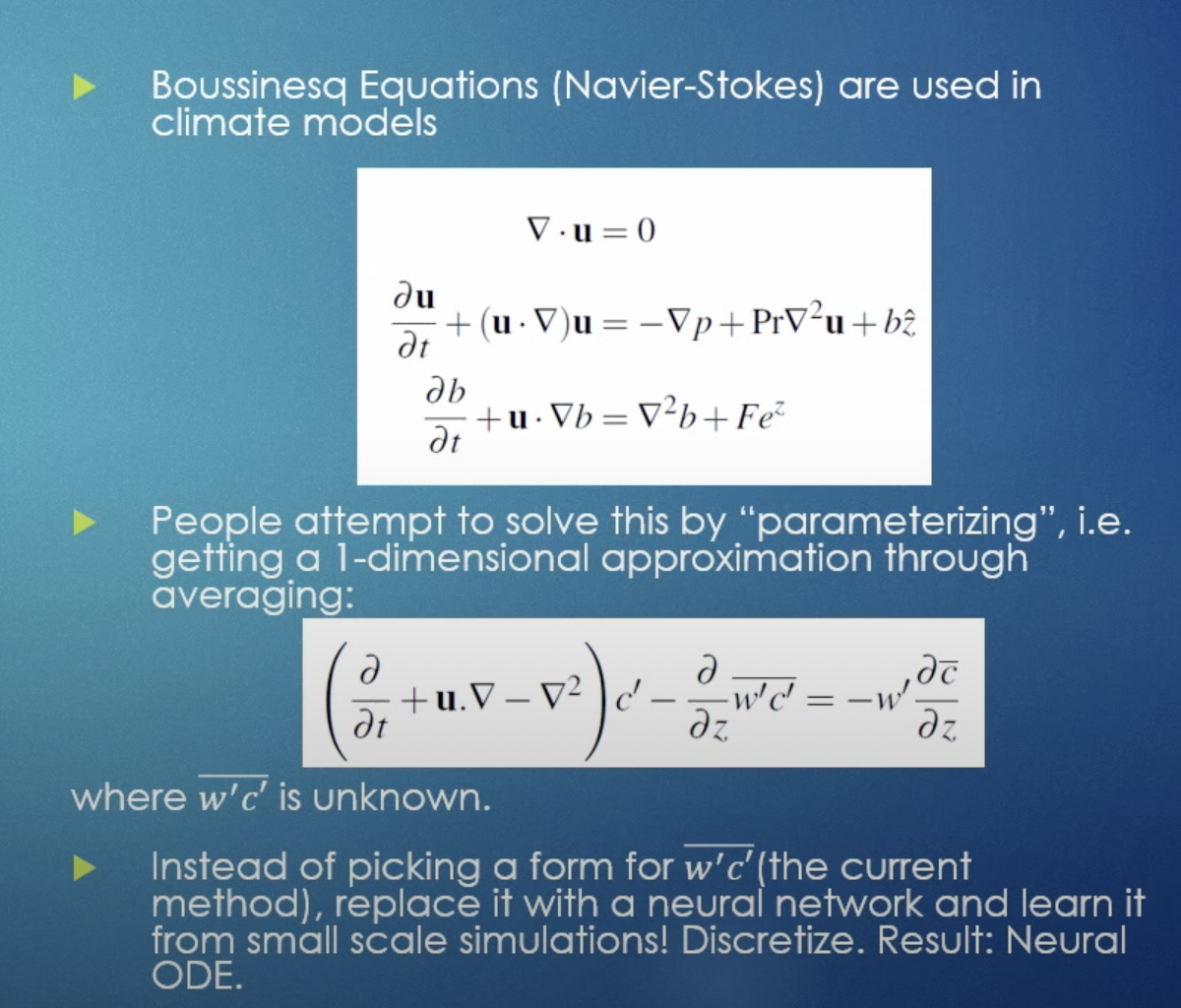
Scaling the software to “real” problems

Neural ODE with batching on the GPU (without internal data transfers) with high order adaptive implicit ODE solvers for stiff equations using matrix-free Newton-Krylov via preconditioned GMRES and trained using checkpointed adjoint equations. See Yingbo Ma’s talk.

using OrdinaryDiffEq, Flux, DiffEqFlux, DiffEqOperators, CuArrays
x = Float32[2.; 0.]|>gpu
tspan = Float32.((0.0f0, 25.0f0))
dudt  = Chain(Dense(2,50,tanh), Dense(50,2))|>gpu
p = DiffEqFlux.destructure(dudt)
dudt_(du, u::TrackedArray,  p, t) = u .= DiffEqFlux.restructure(dudt,p)(u)
dudt_(du, u::AbstractArray, p, t) = u .= Flux.data(DiffEqFlux.restructure(dudt,p)(u))
ff = ODEFunction(dudt_, jac_prototype = JacVecOperator(dudt_,x))
prob = ODEProblem(ff,x,tspan,p)
diffeq_adjoint(p,prob,KenCarp4(linsolve=LinSolveGMRES());u0=x,
  saveat=0.0:0.1:25.0, backsolve=false)

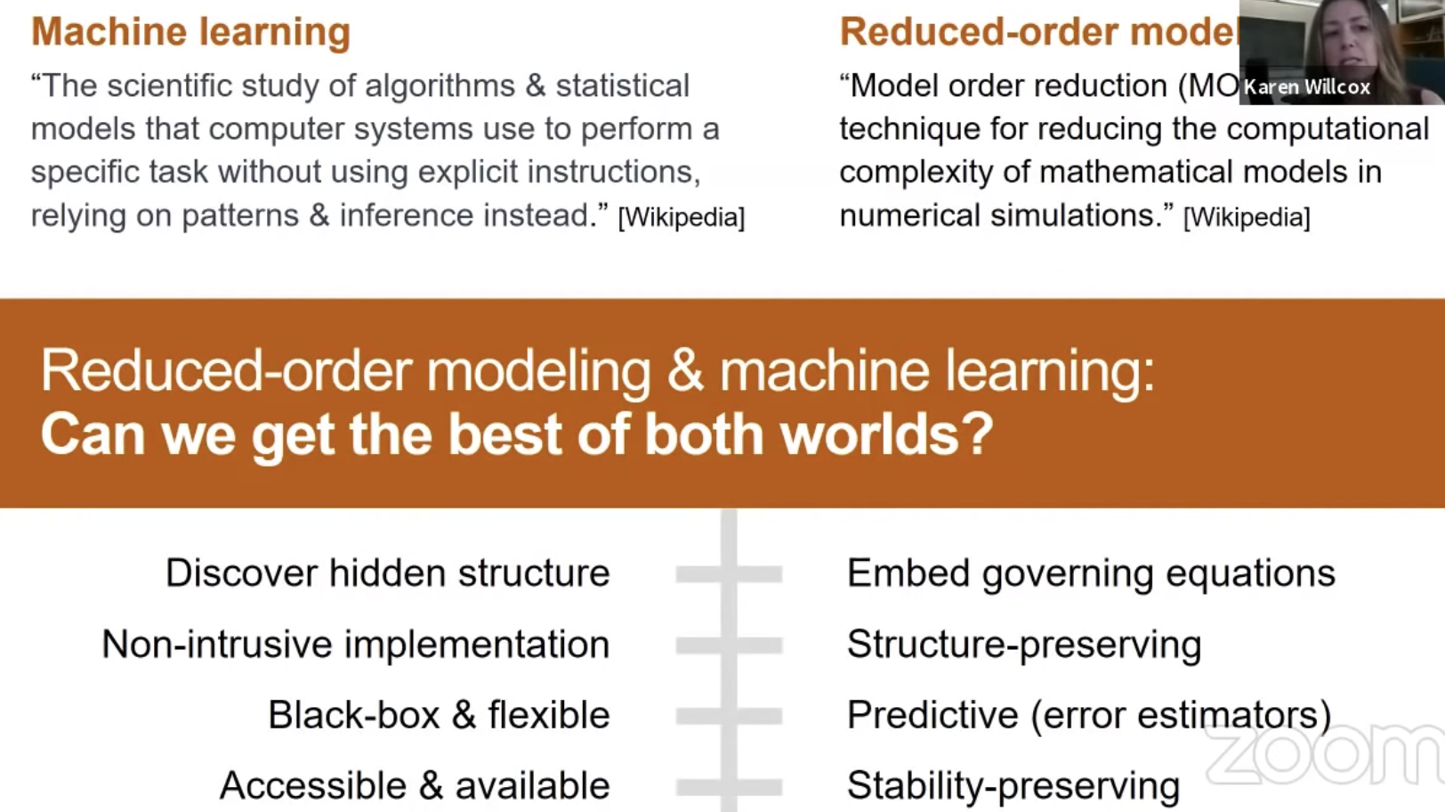
ROM machine learning-燃烧模拟-加速模拟

报告的最后说了一个事实：下面的案例是针对于仿真的，仿真的好处是能拿到不同的参数，然后做降维，这要比实验好做的多。

• 首先对数据的认识非常重要，deeply understand the problem you working with,
• 机器学习算法保证不变量
• 预测chaostis是悬而未决的

https://github.com/Willcox-Research-Group?language=python

参考文献

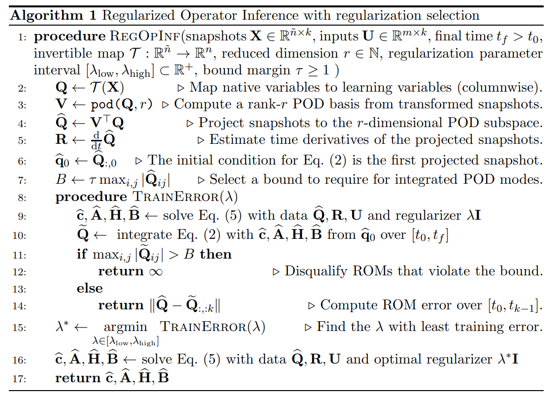
Lift & Learn approach

• Full model

$${d\over dt}q(t)= c+Aq(t)+H(q(t)\otimes q(t))+Bu(t),\\\\ q(t_0)=q_0, t\in[t_0,t_f]$$

H terms are quadratic,

Example:

1. Incompressible N-S
2. Euler equations can be transformed to quadratic form by using pressure, velocity.
3. A nonlinear tubular reactor model

• ROM model：

$${d\over dt}q_r(t)= c_r+A_rq_r(t)+H_r(q_r(t)\otimes q_r(t))+B_ru(t),\\\\ q_r(t_0)=V^T q_0, t\in[t_0,t_f]$$

Where, $c_r = V^Tc, A_r = V^TAV, H_r=V^TH(V\otimes V), B_r= V^TB$

• Learn model fram data (data driven regression approach) $${d\over dt}\hat{q}(t)= \hat{c}+\hat{A}\hat{q}(t)+\hat{H}(\hat{q}(t)\otimes \hat{q}(t))+\hat{B}u(t),\\\\ \hat{q}(t_0)=V^Tq_0, t\in[t_0,t_f]$$ Solve least-squares problem:（最小二乘法） $$min_{\hat{c},\hat{A},\hat{H},\hat{B}}\sum_{j=0}^{k-1} \left\Vert \hat{c} +\hat{A} \hat{q_j} +\hat{H}(\hat{q}_j\otimes \hat{q}_j) +\hat{B}u_J -\dot{\hat{q}}\right\Vert_2^2$$ 最终，将上式表达为： $$min_{O} \left\Vert DO^T - R^T \right\Vert_F^2\\\\ O = [\hat{c} \space \hat{A} \space \hat{H} \space \hat{B}]\in R^{r\times d(r,m)},(unknown \space opertor)\\\\ D=[1_k \space \hat{Q}^T \space (\hat{Q}\times \hat{Q})^T \space U^T]\in R^{r\times d(r,m)}, (known \space data)\\\\ \hat{Q} =[\hat{q}_0 \space \hat{q}_1 ... \hat{q}_{k-1}]\in R^{r\times k}, (snapshots)\\\\ R = [\dot{\hat{q}}_0 \space \dot{\hat{q}}_1 ...\dot{\hat{q}}_{k-1}]\in R^{r\times k}, (time \space derivatives)\\\\ U = [u_0 \space u_1 ... \space u_{k-1}]\in R^{m\times k} (input)$$ Thus to compute the ROM operators $\hat{c}, \hat{A}, \hat{H}, \hat{B}$ without explicit acess to the original high-dimensional opertor $c, A, H, B$.

• Tikhonov Regularization to alleviate overfitting the operators to the data 参考 $$min_{o_i} \left\Vert Do_i -r_i \right\Vert_2^2 + \left\Vert \Gamma o_i\right\Vert_2^2 = \left\Vert [D ; \Gamma]o_i - [r_i;0]\right\Vert, i=1,..,r$$ $\Gamma$ is a full-rank regularizer.

L2 regularizer $\Gamma = \lambda I$, deriving the ROM toward the globally stable system ${d\over dt}\hat{q}(t)=0$.

• Combustion dynamics $${\partial \vec{q_c}\over \partial t} + \nabla\cdot(\vec{K}-\vec{K}_v) =\vec{S}\\\\ \vec{q}_c = [\rho \space \rho v_x \space \rho v_y \space \rho e\space \rho Y_1 \space \rho Y_2 \space \rho Y_3 \space \rho Y_4]^T$$ $\vec{K}$ the inviscid flux terms, $\vec{K}_v$ the viscous flux terms, $\vec{S}$ is the source terms. $\rho$ density, $Y_l$ is the species mass fraction. CH4 + 2 O2 —> 2 H2O+ CO2.

仿真模型参考：https://github.com/cwentland0/pyGEMS_1D

FLOW MODELING WITH MACHINE LEARNING

• dimensionality reduction

  Dimensionality reduction involves extracting key features and dominant patterns that may be used as reduced coordinates where the fluid is compactly and efficiently described (Taira et al. 2017). 参见⁵

  

• Detecting von Karman-type wakes with hydrodynamic sensors⁶

Machine Learning Based Detection of Flow Disturbances Using Surface Pressure Measurements⁷

利用叶片表面的压力数据$\triangle C_p = 2(p^+ - p^-)/(\rho U^2)$通过机器学习特征-吸力面的来流相对叶片的角度，定义为critical leading-edge suction parameter (LESP)。Using a combination of convolutional and recurrent neural networks.

离散涡方法 代码

将叶片的流场用一个个涡团来近似模拟，但对于有厚度的叶片需要进行修正，考虑kutta条件(zero vorticity at the trailing edge)。

the coordinate along the plate：

$$x = {c\over 2}(1-cos\theta)$$

对于薄翼模型，其涡量分布 bound vortex sheet strength on the plate 有如下简化形式：

$$\gamma(\theta,t)=2U[A_0(t){1+cos\theta\over sin\theta}+\sum_{n=1}^\infty A_n(t)sin(n\theta)],\\\\ x= {c\over 2}(1-cos\theta)$$

对于有一定厚度的翼型，简化满足速度平行于边界的条件:

$$A_0(t) = -{1\over \pi} \int_0^\pi {W(x,t)\over U}d\theta,\\\\ A_n(t) = {2\over \pi} {W(x,t)\over U}cos(n\theta) d\theta$$

无滑移可能通过离散涡方法求解, 最终求得流场速度：

$$W(x,t)= {\partial \phi_B \over \partial z} = {\partial \eta \over \partial x}(U cos\alpha + \dot{h} sin\alpha + {\partial \phi_{lev}\over \partial x} + {\partial \phi_{tev}\over \partial x})\\\\ - U sin \alpha - \dot{\alpha}(x-ac) + \dot{h} cos\alpha - {\partial \phi_{tev}\over \partial z} -{\partial \phi_{lev}\over \partial z}$$

其中，$\phiB, \phi{\lev}, \phi_{tev}$为velocity potentials associated with bound, leading-edge and trailing-edge vorticity. $\eta$ is the camber distribution on the aerofoil. potentials的偏微分分别为垂直于弦的速度。

Kelvin’s 环量守恒：

$$\Gamma_b(t) + \sum_{m=1}^{N_{tev}} \Gamma_{tev_m} + \sum_{m=1}^{N_{lev}} \Gamma_{tev_n} =0,\\\\ \Gamma_b = Uc\pi [A_0(t)+ {A_1(t)\over 2}]$$

Critical leading-edge suction parameter (LESP)

无量纲参数，$LESP(t)=A_0(t)$

LSEP和前缘分离涡初始点之间的联系

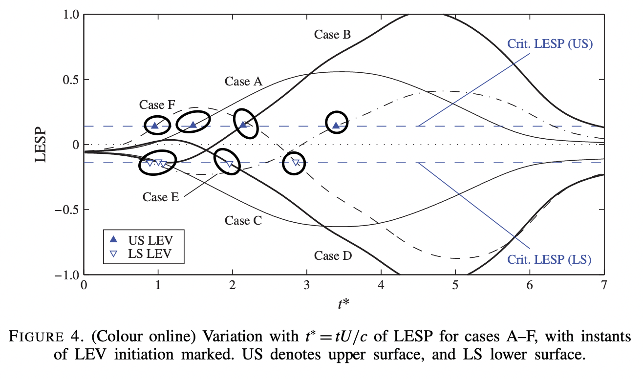
如此神奇，这些初始分离点竟然都在LESP的同一条线上，也就是说，分离点的位置与LESP-$A_0$直接相关。这个结果为Ramesh团队在JFM-2014上发表⁸。这个结果证明了，LESP临界点只跟给定的翼型攻角$\alpha$和雷诺数$RE$有关系。

理论很丰满，但实际工程遇到的问题却很骨感。上面的案例是简化的离散涡模型的结果，但实际问题是非线性的，来流复杂，可压条件，攻角和雷诺数也是随时间变化，因此临界LESP也在变化，直接影响LEV的分离，LEV的分离又对叶轮机械系统的稳定性非常动摇。传感器可以实时获取叶片壁面的动压数据，是否可以用该数据来训练，预测攻角，LESP和其临界点。

如何从压力数据训练LESP？

来自California的Wei Hou⁷就拿这个离散涡的模型做了一些数据训练尝试，虽然没拿实际问题的数据。他们提前改变了模型的预设参数$LESP_c(t)$和$\alpha(t)$, 让其随时间变化。然后，通过离散涡模型仿真，收集叶片表面的压力数据，利用这个数据拿前面已知的参数标签做机器学习，再利用训练好的模型，预测下一个时间点的这两个标签。

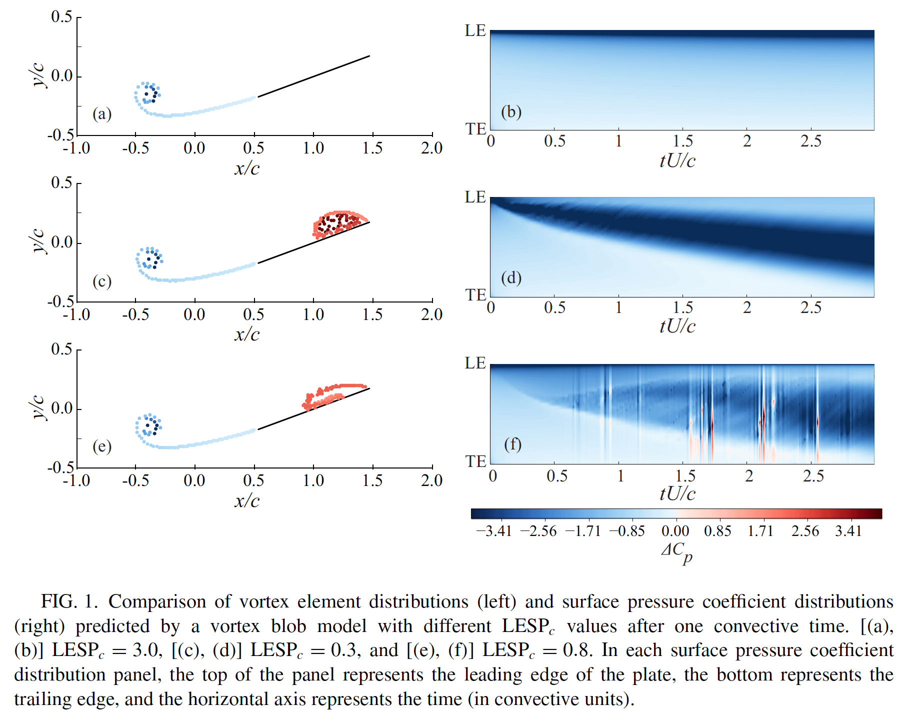
参见2018-pyhsical review fluid-Darakananda ⁹

“This question may appear superficially simple to address since the LESP itself is due directly to pressure, and in fact—as we will discuss below—is proportional to the lowest Fourier mode on the plate surface. However, it is important to remember that in the high-amplitude cases of interest in this work, the flow response (and the surface pressure) is non-linearly dependent on the disturbed critical LESP, so that the surface pressures along the airfoil chord are not trivially related to the leading-edge suction.”

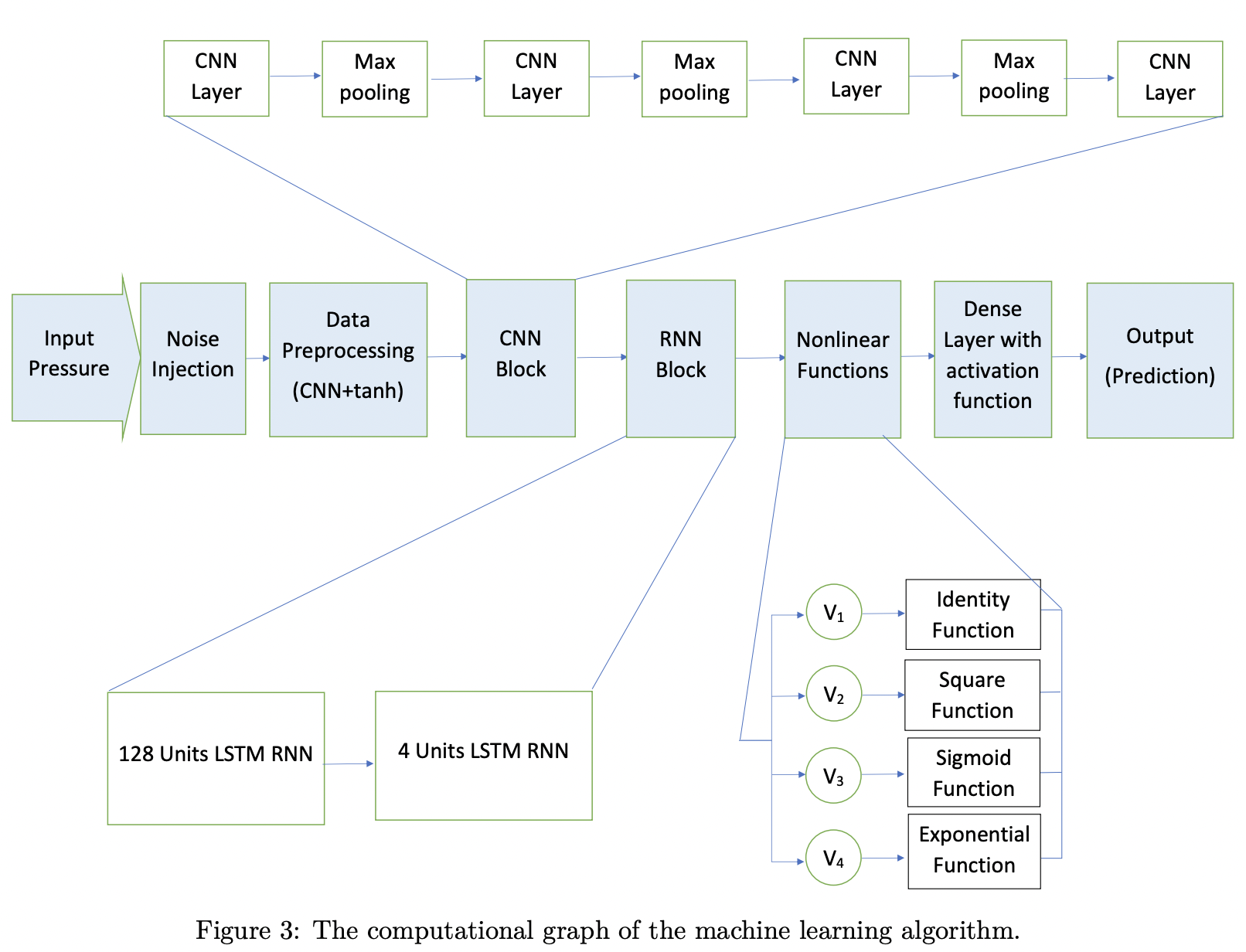
输入矩阵$R^{M*N}$:压力数据采样M=126个点，在叶片上为chebshev分布。N=201为时间序列, 时间间隔为$\triangle t U/c=0.01$.

输出矩阵$R^{1*N}$，为LESP。

The CNN contains 16 separate filters,each utilizing a 5×5 tile of weights, so that the output of this layer is of size $R^{16 126 201}$

learned the functional relationship betweensurface pressures and the LESP and the angle of attack histories by machine-learned systemidentification(MLSID).

assume that the dynamics of the angle ofattack can be described by a linear system of first order differential equations with forcing:

$$\dot{x} = A(p,\tilde{p})x+ u(p,\tilde{p})$$

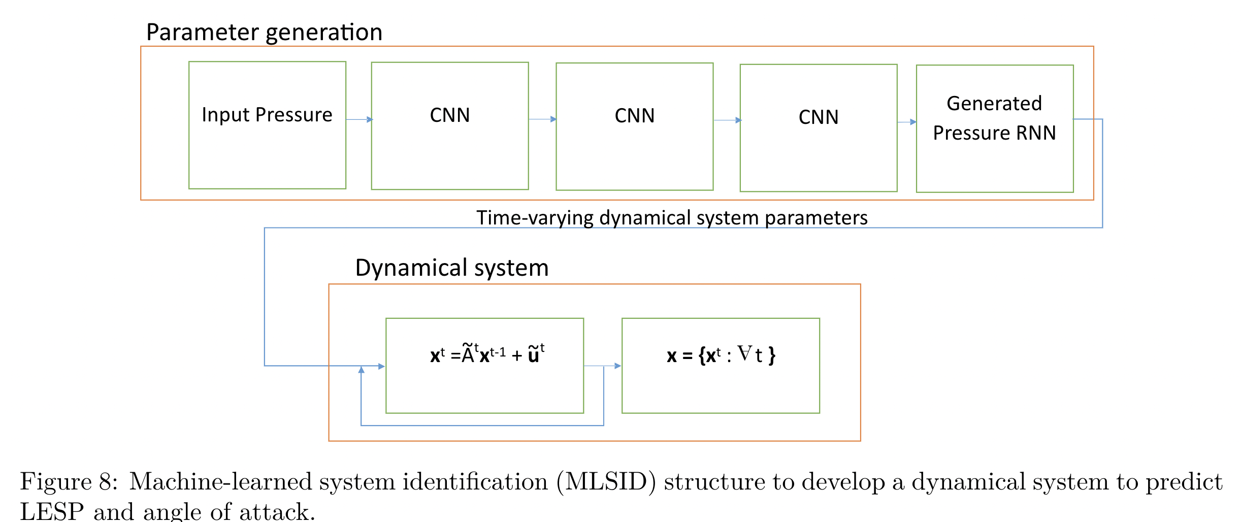
接下来，还可以利用评估得到的LESP做一些事情，简化模型，提取最主要的信息。

Applying the EnKF to a vortex model⁹

准备的数据：The state vector of our EnKF-assisted vortex model consists of the positions and strengths of the n vortex blobs, as well as the current estimate of the LESPc:

$$x_{k-1}:=[x_{k-1}^1 \space y_{k-1}^1 \space \Gamma_{k-1}^1 \space ... \space x_{k-1}^n \space y_{n-1}^n \space \Gamma_{k-1}^n \space LESP_{k-1}^c]^T$$

The nonlinear state transition function $f_k$ propagates the state from step k-1 to step k by the following methods:

(1) computing the bound vortex sheet strength on the plate from the no-penetration condition, using the current vortex blob positions and strength;

(2) computing the volocities of the vortex blobs;

(3) advecting the plate and the vortex blobs;

(4) applying the vortex aggregation algorithm, reducing the strength of any aggregated blobs to zero instead of completely removing the blob;

(5) releasing a new vortex blob from each edge of the plate with strengths based on the Kutta condition at the trailing edge and the current estimate of the LESP_c at the leading edge.

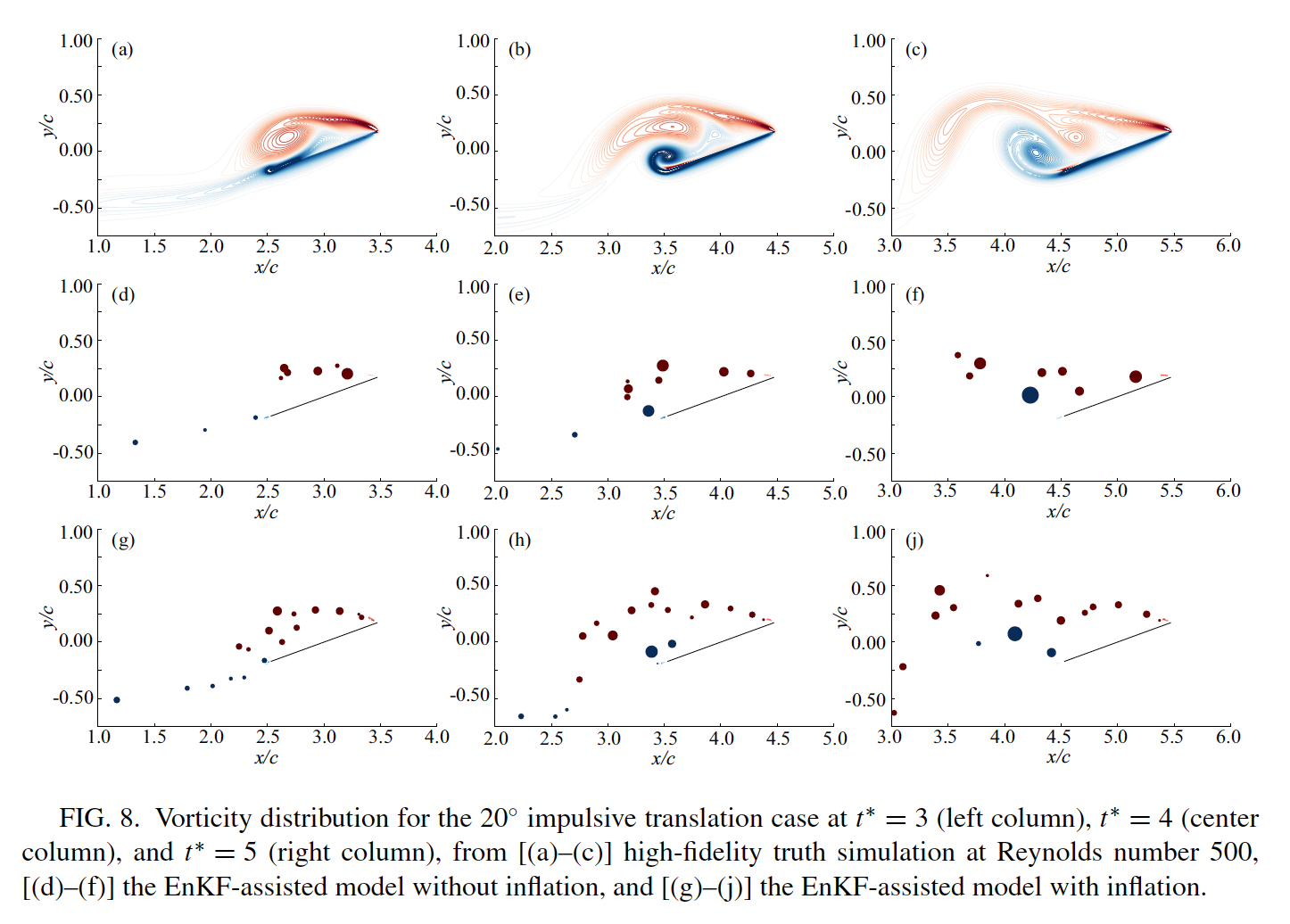
这篇文章的作者也被我挖坟挖到了，真的牛逼的人有个共同的分享精神。Julia写的，之前接触过一些，挺优美的语言。

Deep neural networks for waves assisted by the Wiener–Hopf method 学习笔记-黄迅

$$\psi_s(x, r)= {w^2\over 2\pi}\int_{-\infty}^{+\infty} \beta(\mu, r)e^{i w\mu x}d\mu = A_{mn}{w^2\over 2\pi} \underbrace{\int_{-\infty}^{+\infty} G_{mn}(\mu,r)e^{iw\mu x}d\mu}_{G_{mn}}$$ $$\psi_s(x,r) = \sum_{m=-m_\infty}^{m_\infty} \sum_{n=1}^{n_\infty}A_{mn}G_{mn}+n$$

训练数据准备：

10000 items: $\psis$ of various (m,n) with random amplitudes $A{mn}$ ,

这个例子实际较为简单，可以用来作为benchmark。

训练 differenatial operator

笔记2: 针对有物理限制的案例

之前的案例讨论的都是如何训练神经网络使得近似operator。但是如果有边界条件存在的情况，我们又该如何取舍？

分析1:

详细见：https://github.com/cics-nd/pde-surrogate

$$\mathcal{N}(u(s);K(s))= f(s), s\in\mathcal{S},\\\\ \mathcal{B}(u(s)) = b(s), s\in \Gamma$$

$\mathcal{B}$ 是PDE的边界条件。

Darcy flow：

$$-\nabla \cdot (K(s)\nabla u(s))= f(s), s\in \mathcal{S}\\\\ with \space boudnary: u(s)=u_D(s), s\in\Gamma_D\\\\ \nabla u(s)\cdot n = g(s) s\in \Gamma_N$$

该案例最终可以转化为求最优化问题：

$$arg min_u V(u;K)$$ $$L(\theta;{x^{i}}_i^N)= {1\over N}\sum_{i=1}^N[V(\hat{y}_\theta(x^i), x^i)+\lambda B(\hat{y}_\theta(x^i))]$$

$\lambda$ is the weight (Lagrange multiplier) to softly enforce the boundary conditions.

限制是好事：

如果没有限制，predict 一段时间就会跑偏，有了限制（前提已知），就会神经网络就会自己主动调整，预测正确的结果。

利用卷积-encoder-deconder neural network ，跟SVD有联系。

分析2:

详细见：https://github.com/maziarraissi/DeepVIV

作者主页：https://maziarraissi.github.io/research/

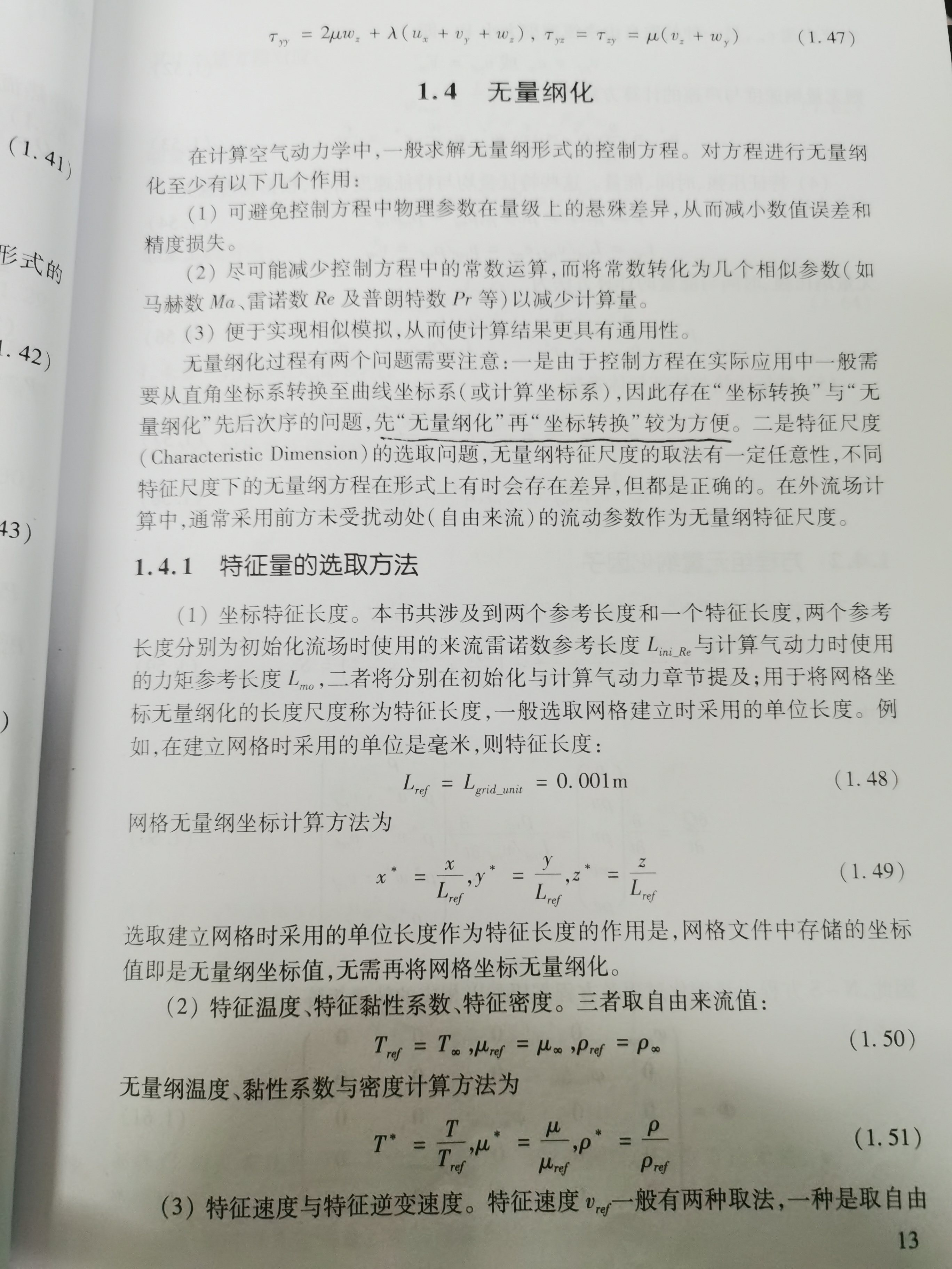
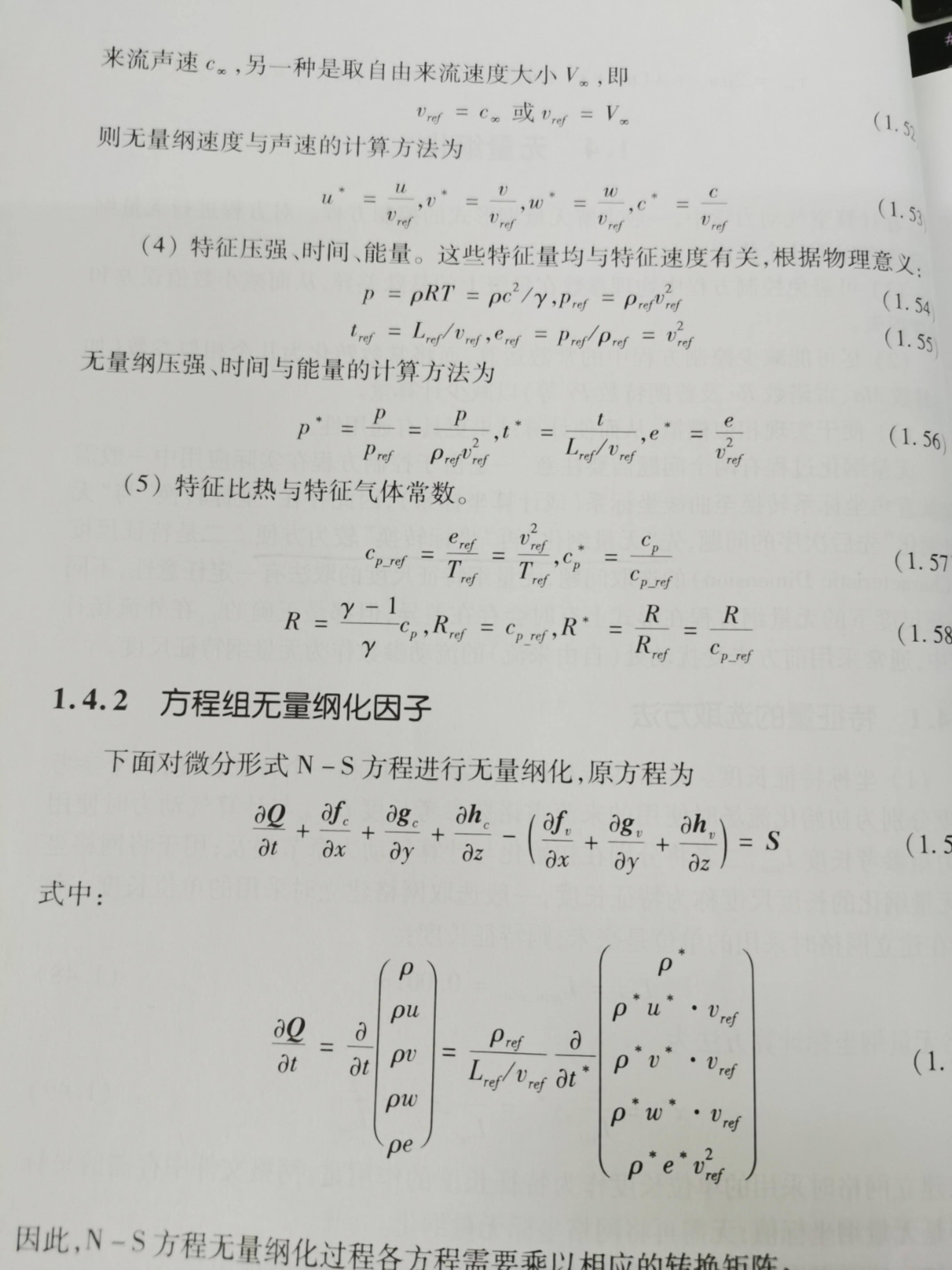
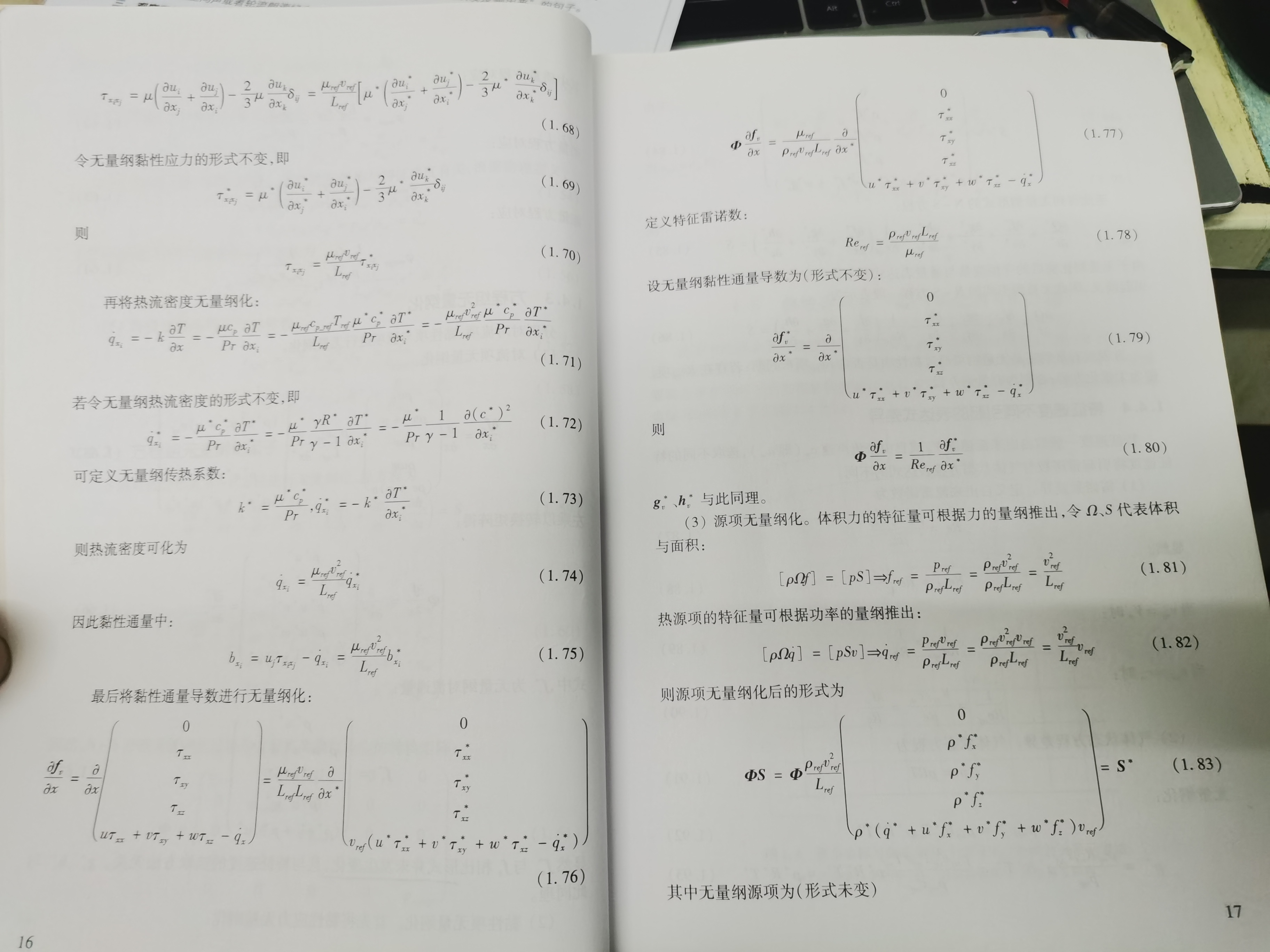
无量纲处理 实际仿真数据

参考

¹. [2019 SIAM Conference on Applications of Dynamical Systems ↩

². https://github.com/pvlachas/RNN-RC-Chaos ↩

⁴. Backpropagation Algorithms and Reservoir Computing in Recurrent Neural Networks for the Forecasting of Complex Spatiotemporal Dynamics ↩

⁵. Machine Learning for Fluid Mechanics ↩

⁶. Detecting exotic wakes with hydrodynamic sensors Mengying Wang and Maziar S. Hemati ↩

⁷. AIAA conference-2019,Machine Learning Based Detection of Flow Disturbances Using Surface Pressure Measurements Wei Hou∗1 , Darwin Darakananda†1 , and Jeff D. Eldredge‡1 ↩

⁸. Kiran Ramesh, Ashok Gopalarathnam, Kenneth Granlund, Michael V. Ol, and Jack R. Edwards. Discrete-vortex method with novel shedding criterion for unsteady aerofoil flows with intermittent leading-edge vortex shedding. Journal of Fluid Mechanics, 751:500–538, 2014 ↩

⁹. Data-assimilated low-order vortex modeling of separated flows,PHYSICAL REVIEW FLUIDS 3, 124701 (2018) ↩

¹⁰. 2017- APPLIED MATHEMATICS Data-driven discovery of partial differential equations Samuel H. Rudy1,*, Steven L. Brunton2, Joshua L. Proctor3 and J. Nathan Kutz1 ↩

¹¹. Universal Differential Equations for Scientific Machine Learning Christopher Rackauckasa - 2020-10-10 ↩