DMD

DMD 算法汇总

• POD
• standard DMD
• On-line DMD
• Hankel-DMD
• Koopman mode decomposition

持续更新中。。

POD

realization of a stationary stochastic process and therefore can use statistical tools such as POD to obtain a meaningful decomposition. POD is a linear decomposition of the flow field into spatially orthogonal modes and uncorrelated temporal coefficients.

the chaotic component $u_c(x,y,t)$ 可以分解：

$$u_c(x,y,t)= \sum_k a_k (t)\phi_k(x,y)$$

其中， $\phi_k$ 为POD 模态³, $a_k$ 与时间相关。

DMD 或 Koopman decomposition mode, could evolve exponentially with time. POD 模态 互相空间正交，DMD 不必。POD provide a robust representation of post-transient chaotic components since the modes become independent of the initial condition due to 遍历性.

在该³文献中，Koopman modes 和 POD 模态同时使用，the most economical choices for constructing low-dimensional approximations of the quasi-periodic and chaotic components of the flow respectively.

$$u_{n_k,n_p}(x,t)= \sum_{j=1}^{n_k} u_j(x)e^{i w_j t} + \sum_{l=1}^{n_p} \phi_l(x)a_l(t)$$

stack the modes by starting from the Koopman modes (including the mean flow) in the order of decreasing energy and then use the POD modes of the chaotic component with the same order.

standard DMD

$$x_{j+1}=F(x_j)$$ $$X_k=[x_1 \space x_2 \space ... \space x_k],Y_k=[y_1 \space y_2 \space ... \space y_k],$$ $$J_k =\sum_{i=1}^{k} ||y_i -A_k x_i||^2 = ||Y_k - A_k X_k||^2_F$$

where $F$ denotes the Frobenius norm on matrices. The unique minimum-norm solution to this least-squares problem is given by

$$A_k=Y_k X_k^+$$

where $X_k^+$ denotes the Moore-Penrose pseudoinverse of $X_k$.

Here, we shall assume that $X_k$ has full row rank, in which case $X_k X_k^T$ is invertible, and

$$X_k^+ = X_k^T (X_k X_K^T)^{-1}$$

The $A_k$ given above is the unique solution that minimizes $J_k$.

Consider minimizing a modified cost function:

$$\tilde{J_k} = \sum_{i=1}^k \rho^{k-i} ||y_i - A_k x_i||^2$$

where $0<\rho \leqq 1$.

On-line DMD¹

这个算法特别适合实验数据测点数n比较小，而时间t非常大的实时迭代更新.

一般一个snapshots的展开的列数相对较大，但snapshot数较少. 为了满足实时性计算性能要求，参考文献提出了类似于classical recursive least-squares estimation algorithm recursive least-squares algorithm update a vector in real time.

首先，将上面$A_k=Y_k X_k^+$改写为

$$A_k = Y_k X_k^T (X_k X_k^T)^{-1}= Q_k P_k$$

那么，为了计算下个时间步的$Ak$，则需要更新$Q{k+1}$和$P_{k+1}$

$$Q_{k+1}= Y_{k+1}X_{k+1}^T = [Y_k \space y_{k+1}][X_k \space x_{k+1}]^T = Y_k X_k^T + y_{k+1}x_{k+1}^T\\\\ P_{k+1}^{-1}= X_{k+1}X_{k+1}^T =[X_k \space x_{k+1}][X_k \space x_{k+1}]^T= X_kX_k^T + x_{k+1}x_{k+1}^T$$

上述公式说明了，可以通过单单更新rank-1来找到下一个时间不的Q和P矩阵。

$$Q_{k+1}= Q_k + y_{k+1}x_{k+1}^T\\\\ P_{k+1}^{-1}=P_k^{-1} + x_{k+1}x_{k+1}^T$$

这样就可以更新下个时间步的DMD矩阵：

$$A_{k+1}=Q_{k+1}P_{k+1}^{-1}=(Q_k + y_{k+1}x_{k+1}^T) (P_k^{-1} + x_{k+1}x_{k+1}^T)^{-1}$$

计算$P_k^{-1}$还要设计到求逆，这是非常耗时的，$O(n^3)$. 可以通过Sherman-Morrision formula进行简化²

$$\cssId{Overlinev}{(A+ uv^T)^{-1}} = A^{-1} - {A^{-1}uv^T A^{-1}\over 1+v^T A^{-1}u}$$

把上面$\href{ #Overlinev}{公式}$ 应用到P

$$P_{k+1}= (P_k^{-1}+ x_{k+1}x_{k+1}^T)^{-1} = P_k - {P_k x_{k+1}P_k \over1+x_{k+1}^T P_k x_{k+1}}$$

令

$$\gamma_{k+1}={1 \over1+x_{k+1}^T P_k x_{k+1}}$$

因此：

$$A_{k+1}= (Q_k + y_{k+1}x_{k+1}^T) ( P_k - \gamma_{k+1} {P_k x_{k+1}P_k })\\\\ = Q_kP_k - \gamma_{k+1}Q_k P_k x_{k+1}x_{k+1}^T P_k \\\\ + y_{k+1}x_{k+1}^T P_k- \gamma_{k+1}y_{k+1}x_{k+1}^T P_k x_{k+1}x_{k+1}^T P_k$$

简化last two terms，

$$y_{k+1}x_{k+1}^T P_k- \gamma_{k+1}y_{k+1}x_{k+1}^T P_k x_{k+1}x_{k+1}^T P_k = \gamma_{k+1}y_{k+1}(\gamma_{k+1}^{-1}-x_{k+1}^TP_k x_{k+1})x^T_{k+1}P_k\\\\ = \gamma_{k+1}y_{k+1}x^T_{k+1}P_k$$

所以：

$$A_{k+1} = A_k - \gamma_{k+1}Q_k P_k x_{k+1}x_{k+1}^T P_k + \gamma_{k+1}y_{k+1}x^T_{k+1}P_k$$

• 解释：更新A的过程可以看成 将$y{k+1}-A_kx{k+1}$的误差用于更正$A_{k+1}$.
• $Ak x{k+1}$ 和 $Pk x{k+1}$大概需要$4n^2$floating-point. 而 standard DMD 为 $O(kn^2

• 思考: 这个获取可以用在DMD旋转失稳的旋转速度的捕捉，随着工况的变化，该速度一直在变化，也带来了频率的变化。

  可以用来作失速前的预警。

目前有做过尝试，但是由于time-delay的限制，效果不明显。

Hankel-DMD

Calculate the Koopman spectrum is to apply DMD to Hankel matrix of data. The Hankel matrix is created by the delay-embedding of time series measurements on the observables. Delay-embedding is an established method for geometric reconstruction of attractors for nonlinear systems based on measurements of generic observables.

Connection between linear analysis of delay-embedded data and identification of nonlinear systems using the Koopman linear analysis.

projections of data vectors converge to function projections in the space of observables.

new connection between the SVD and POD on the ensemble of observables on ergodic dynamical systems.

Koopman mode decomposition ⁴

首先从基本的N-S方程的简化形式出发：

$$\partial_t u(x,t)=F(u(x,t))$$ $$g^{\tau}(u(x,t)):= U^\tau g(u(x,t))= g(u(x,t+\tau))$$

g 表示可观，$U^\tau$ denotes maps the function g to a new function $g^\tau$., 为线性算子。所以，通过spectrum和特征值可以了解系统的运行机制。Koopman 特征值具有以下特性：

$$\phi^{\tau}(u): = U^\tau \phi_j(u) = e^{\lambda_j \tau}\phi_j (u)$$

The Koopman freuqencies, $w_j$:

$$\lambda_i = iw_j, w_j \in R$$

假定所有可观测的数据全部收敛到Koopman特征函数上，

$$g(u)= \sum_{j=1}^{\infty}g_j \phi_j (u)$$

最后形成Koopman mode decomposition 的基本表达：

$$g^{\tau}(u):= U^{\tau} g(u) = \sum_{j=1}^\infty g_j \phi_j(u)e^{i w_j \tau}$$

The vector $g_i$ called the Koopman mode assosiated with the Koopman frequency $w_j$, describes the components of the observable g obtained by projection of the observable onto the Koopman eigenfunction $\phi_j$.

For chaos behavior, the scalar observable g can be written as

$$U^\tau g = \sum_{k\in Z} g_k \phi_k e^{i k\cdot \Omega \tau} + \int_{-\infty}^{\infty} e^{i\alpha \tau} dE_\alpha (g)$$

Informally speaking, $i\alpha$ with $\alpha \in (-\infty, \infty)$, denotes a continuum of eigenvalues distributed along the imaginary axis. $dE_\alpha(\cdot)$ is the spectral measure of the Koopman operator.

为了更好的应用于flow application, 转化为内积的形式：

$$<g, U^\tau g>_H = \sum_{k=1}^\infty |g_k|^2 e^{i w_k \tau} + \int_{-\infty}^{\infty} e^{i \alpha \tau} \rho+g (\alpha) d\alpha$$

在满足遍历性假设的基础上，有：

$$<g, U^\tau g>_H =r_g(\tau): lim_{T->\infty} {1\over T} \int_0^T g(t)g^*(t+\tau) dt$$

即为g的自相关函数。

因此，we can approximation the spectral density of the Koopman operator by first extracting the chaotic component of g, then approximating $r_g$ using finite-time observations, and finally applying inverse Fourier transform to $r_g$.

$$cov(g, U^\tau g)= \int_{-\infty}^{\infty} e^{i\alpha \tau} \rho(\alpha) d\alpha$$

where $\rho$ is called the Power Speactral Density (PSD) of the stochastic process.

Koopman modes 自然也满足N-S 方程：

$$u_j = \nabla^\perp \psi_j, j=1,2,3$$

其vorticity field

$$\xi_j = \nabla \times u_j, j=1,2,3...$$

• 优于DMD的点在于：可以处理宽带噪声；

三步：

• we apply a high-resolution algorithm - adapted from Laskar- to detect the candidate discrete Koopman frequencies and modes. The Laskar algorithm provides a controllable balance between accuracy and computational efficiency which makes it suitable for large data sets like high-resolution flow snapshots. Moreover, it makes direct use of the harmonic averaging which has proven convergence properties for computation of koopman mode.
• use the ergodic properties of the attractor to discard the spurious frequencies that are artifacts of the continuous spectra.
• After extracting the periodic components of the flow, we estimate the continuous Koopman spectrum by the Welch method to the chaotic residual.1

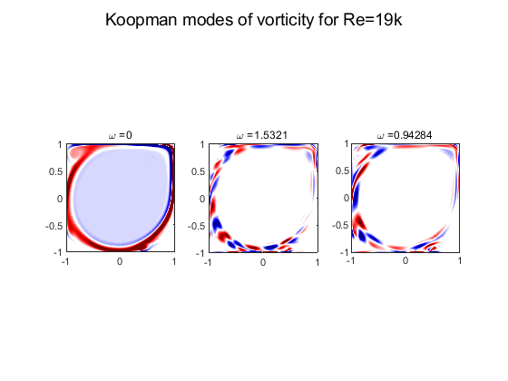
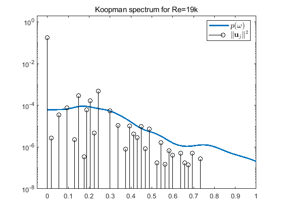
提取离散频率，然后continuous spectra estimator to the remainder.

A. Harmonic averaging and DFT

The koopman modes can be computed via direct projection of observables onto the Koopman eufebfybction, $\phi_j$.

$$g_j : <g,\phi_j>_H=\lim_{T \to \infty} {1\over T} \int_0^T g(\tau) e^{-iw_j \tau}d\tau$$

Assuming uniform sampling at time instants, approximate the harmonic average as

$$g_j^N = {1\over N} \sum_{k=0}^{N-1} g(k)e^{-i w_j\tau_k}g_j^N = {1\over N} \sum_{k=0}^{N-1} g(k)e^{-i w_j\tau_k}$$

The harmonic average of observation by DFT:

$$\hat{g}_j={1\over N} \sum_{k=0}^{N-1} g(k)e^{-i\Omega_j k \triangle \tau}$$

DFT is shown to be equivalent to DMD when applied to a linearly independent sequence of snapshots with zero mean.

对比

标准DMD：前6阶模态

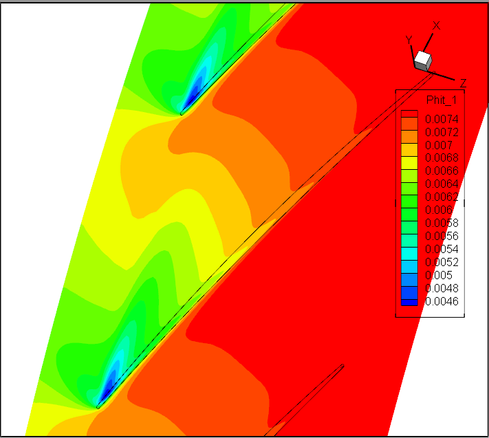
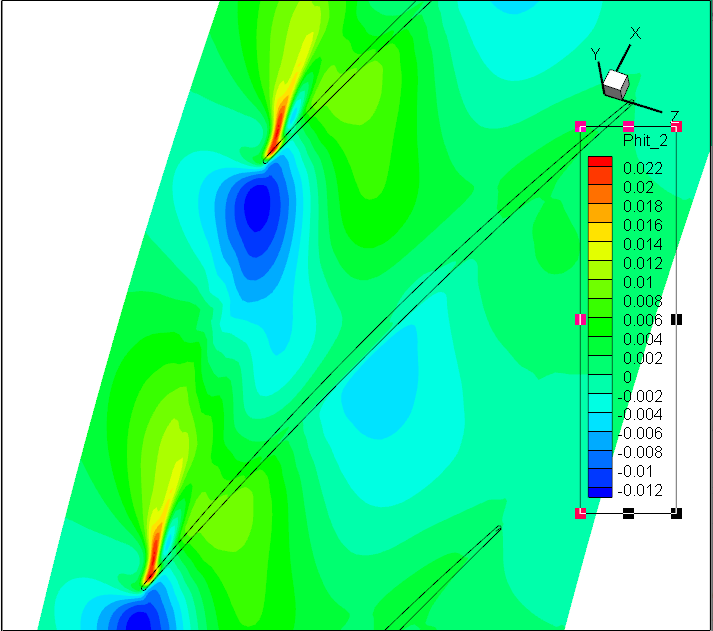
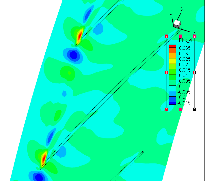
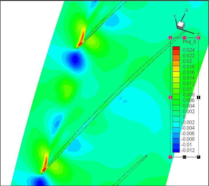
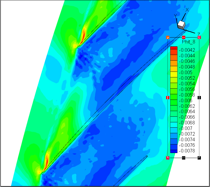
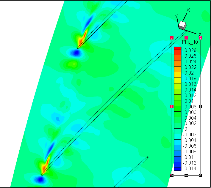
Koopman DMD：前7阶模态Sp

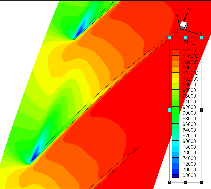
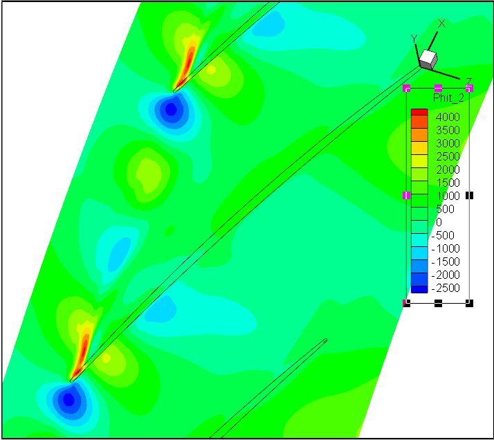
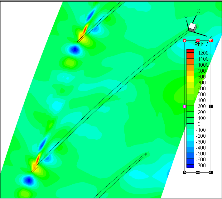
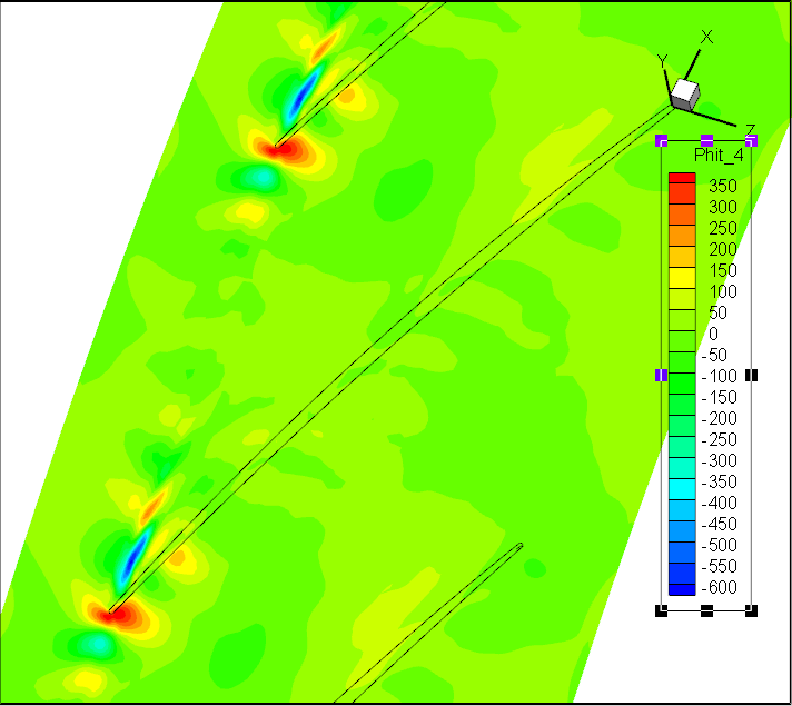
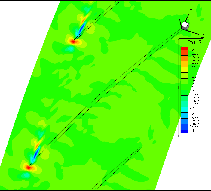
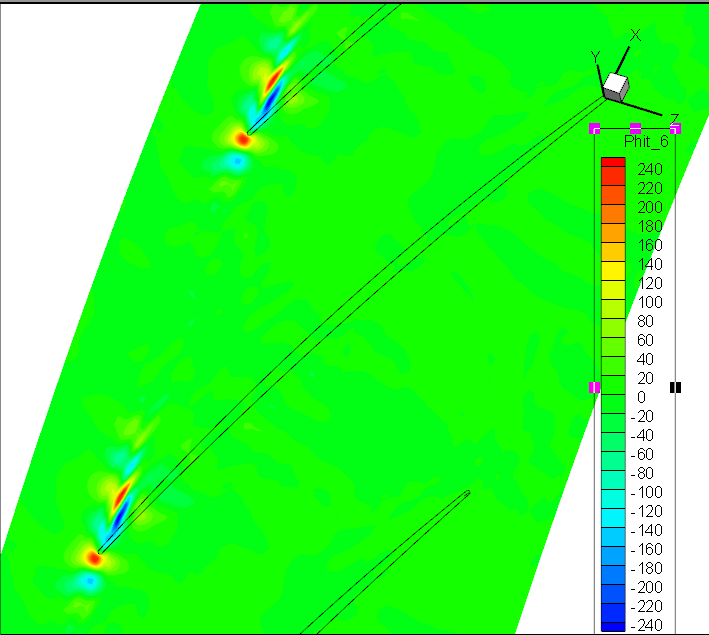
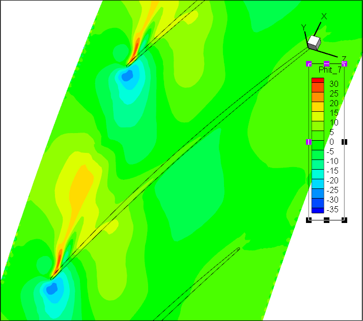
前7阶模态Wm;轴向速度

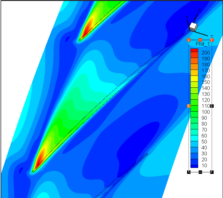
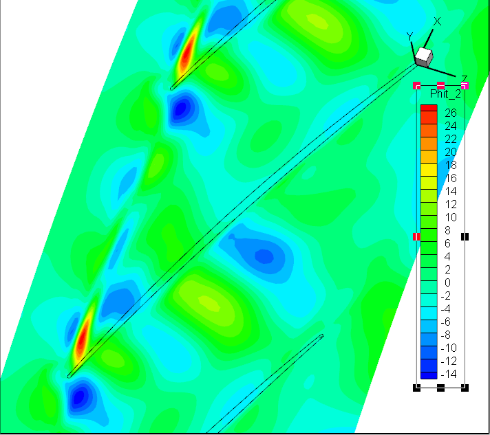
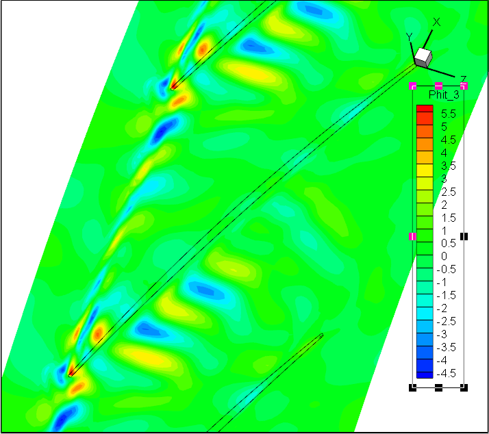
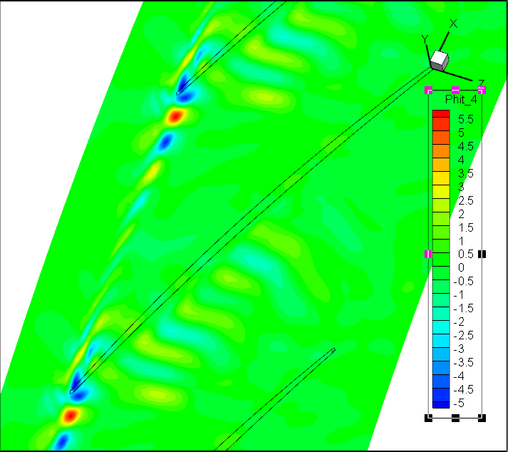
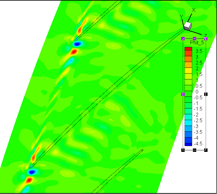
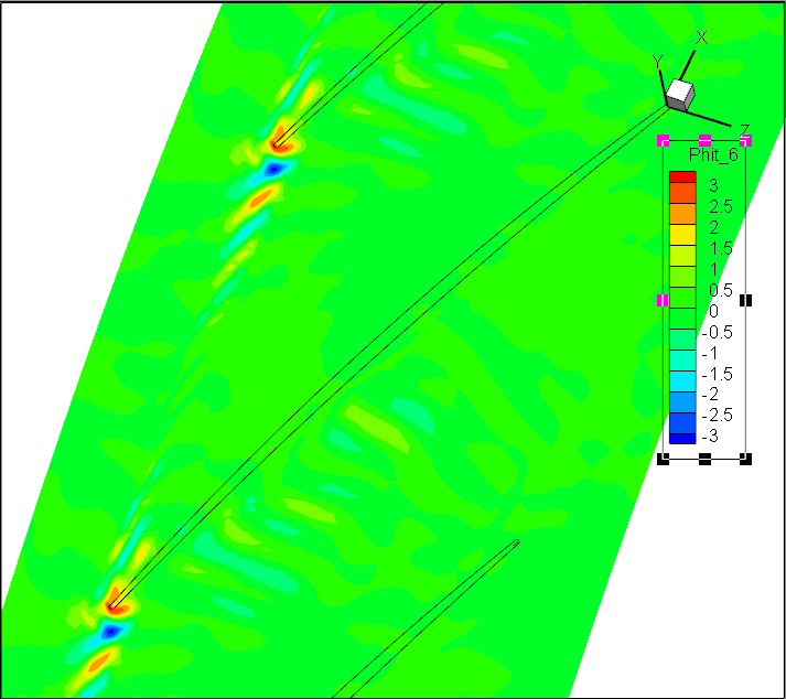
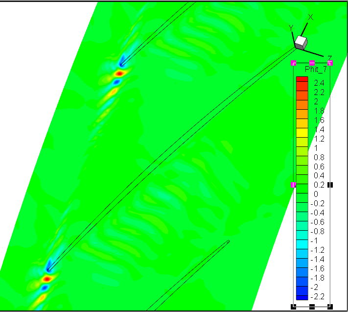
前7阶模态Wr;径向速度

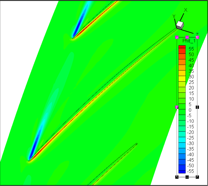
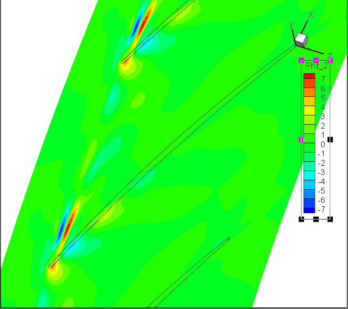
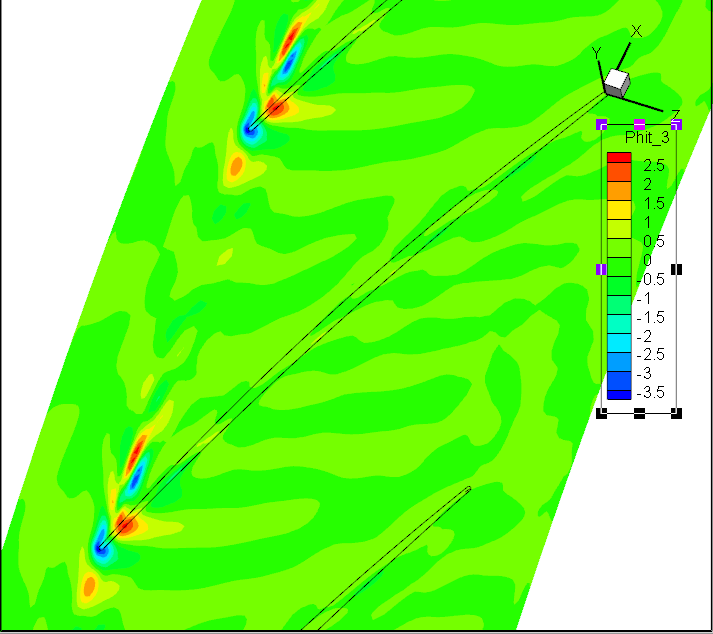
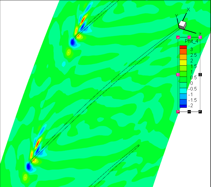
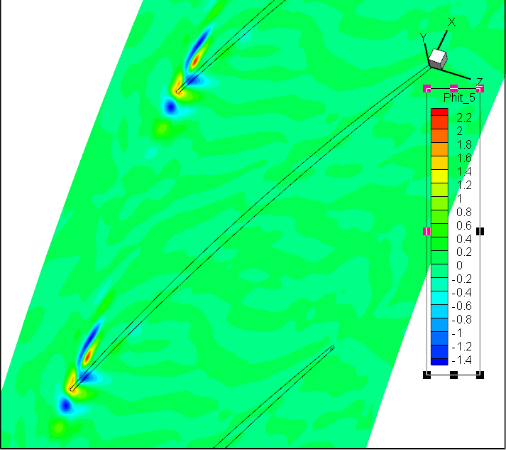
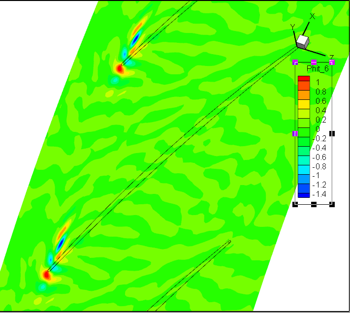
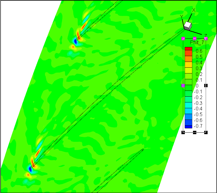
前7阶模态Wt;径向速度

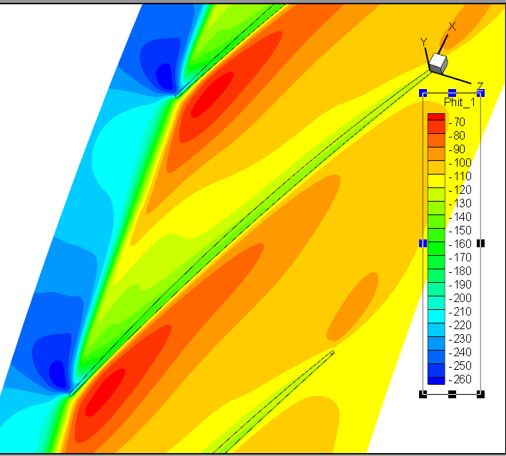
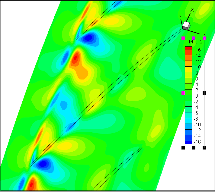
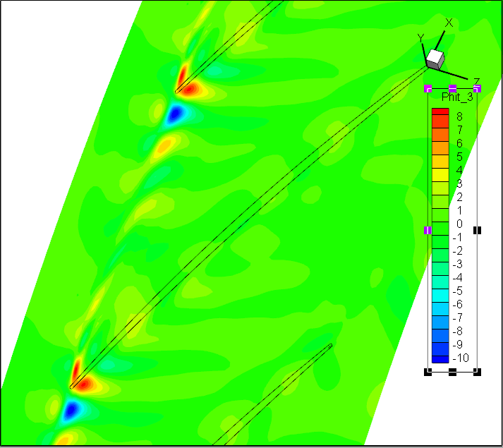
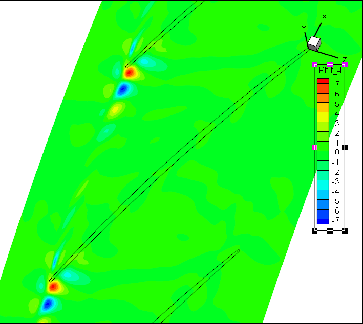
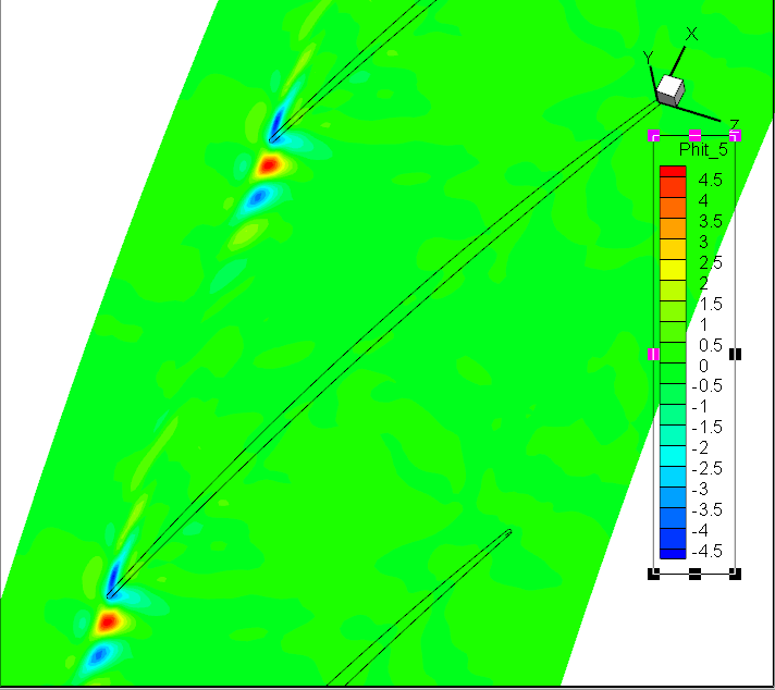
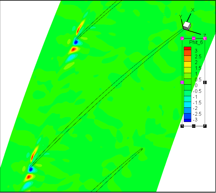
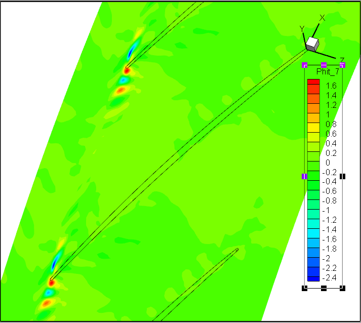
但实验效果不佳!

Hypergraph && mix_norm ⁷

首先需要获得流场的速度场和速度梯度。

• 方法1：

对于non-uniform grid, 利用matlab gridfit 函数近似，将非结构网格转化为等间距矩阵。

接着，参考利用Jacobian matrix：

[dxi,dxj]=gradient(x);
[dyi,dyj]=gradient(y);
[dui,duj]=gradient(u);

then the Jacobian of the transformation is

[dxi dxj
dyi dyj]

the determinant is

DET=dxi.*dyj- dxj.*dyi;

the inverse of the Jacobian has these 4 coefficients:

JAC11=DET.*dxi;
JAC21=DET.*dyi;
JAC12=DET.*dxj;
JAC22=DET.*dyj;

Then to transform the gradient [dui,duj] into dux, duy you just do:

dux=dui.*JAC11+duj.*JAC12;
duy=dui.*JAC21+duj.*JAC22;

• 方法2：无网格法⁸

Basic theory of the WLS meshless methods

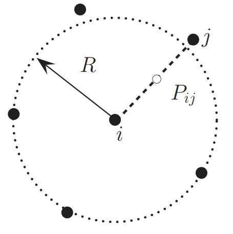
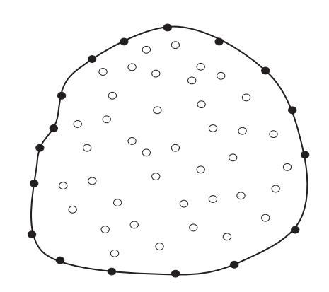
The coordinate difference between the satellite j and the center i can be express as

$$h_j^i = x_j -x_i, l_l^i = y_j -y_i$$

For simplicity, we use $h_j$ and $l_j$ to denote $h_j^i$ and $l_j^i$, respectively. The vector

$$\vec{r}_j^i= (h_j , l_j)$$

starts from i to j, its length is

$$r_j^i = \sqrt{h_j^2 + l_j^2}$$

and the reference radius of cloud as

$$R_i = min(r_1^i, r_2^i, ..., r_j^i, ..., r_{M_i}^i)$$

$M_i$ is the total number of the satellites in the cloud.

The spirit of least-squares method apply Taylor sires about a point $P_i(x_i, y_i)$:

$$f = f_i +a_1 h + a_2 l + {1\over 2}a_3 h^2 +{1\over 2} a_4 l^2 + a_5 hl + O(h^3,l^3)$$

where $f= f(x,y)$ and $f_i = f(x_i,y_i)$ are the function values, $h=x-x_i$ and $l=y-y_i$ are the coordinate differences between the points. The coefficients $a_k(k=1,2,3,4,5)$ represent the partial derivatives of the function at $P_i(x_i,y_i)$:

$$a_1= {\partial f\over \partial x}|_i, a_2={\partial f\over \partial y}|_i, a_3={\partial^2 f\over \partial x^2}|_i, a_4={\partial^2f\over \partial y^2}|_i, a_5= {\partial^2 f\over \partial x\partial y}|_i$$

Keeping the terms until second order, we obtain the approximate function value at Point $P_j(x_j, y_j)$

$$\tilde{f}_j = f_i +a_1 h_j + a_2 l_j + {1\over 2}a_3 h_j^2 +{1\over 2} a_4 l_j^2 + a_5 h_jl_j$$

一阶精度：

$$\tilde{f}_j = f_i +a_1 h_j + a_2 l_j$$

and the error between the exact and approximate value is

$$e_j = f_j - \tilde{f}_j = f_j - (f_i + a_1 h_j +a_2 l_j)$$

A weight function is introduced here to construct $e_j$ considering the effect of different distance between the satellite j and the center i :

$$w_j^i = {r_j^i \over R_i}$$

Then for cloud $C_i$, the total error can be estimated by the following expression:

$$\Phi = {1\over 2}\sum_{j=1}^{M_i}(w_j^i e_j)^2$$

In order to minimize the error, its derivatives about $a_1$ and $a_2$ are set to zero:

$${\partial \Phi\over \partial a_1}={\partial \Phi\over \partial a_2}=0$$

and we gain a set of linear equtions

$$Ax=b$$ $$A= \begin{bmatrix} \sum w_j^{i^2}h_j^2 & \sum w_j^{i^2}h_jh_j \\ \sum w_j^{i^2}h_j l_j & \sum w_j^{i^2}l_j^2 \\ \end{bmatrix}$$

If the matrix A is not singular, this system of equations can be solved by the following simple strategy:

$$x= A^{-1} b$$

The solution can be written into linear combinations of the function values at different points

$$a= {\partial f\over \partial x}|_i = \sum_{j=1}^{M_i} \alpha_j (f_j - f_i),\\\\ a_2 = {\partial f \over \partial y}|_i = \sum_{j=1}^{M_i} \alpha_i (f_j - f_i), a_2 ={\partial f\over \partial y}|_i = \sum_{j=1}^{M_i}\beta_j(f_j-f_i)$$

where, $\alpha_i$ and $\beta_j$ are computed from $A^{-1}$. By removing the dependence of the points i itself in the derivative approximation to satisfy,

$${\partial f \over \partial x}|_i= \sum_{j=1}^{M_i} \hat{\alpha}_j f_j, {\partial f \over \partial y}|_i= \sum_{j=1}^{M_i} \hat{\beta}_j f_j$$

where

$$\hat{\alpha}_j = \alpha_j + \hat{w}_j \alpha_i, \hat{\beta}=\beta_j + \hat{w}_j \beta_i$$

• wlsqm.pdf (old documentation for the old pure-Python version of WLSQM included in FREYA, plus the sensitivity calculation)
• eulerflow.pdf (clearer presentation of the original version, but without the sensitivity calculation)
• wlsqm_gen.pdf (theory diff on how to make a version that handles also missing function values; also why WLSQM works and some analysis of its accuracy)

def main():
    x = np.random.random( (1000, 2) )                # point cloud (no mesh topology!)
    F = np.sin(np.pi*x[:,0]) * np.cos(np.pi*x[:,1])  # function values on the point cloud
    X,Y,Z = project_onto_regular_grid_2D(x, F, fit_order=2, nk=30)
    plot_wireframe( {"x" : (X, r"$x$"),
                     "y" : (Y, r"$y$"),
                     "z" : (Z, r"$f(x,y)$")} )

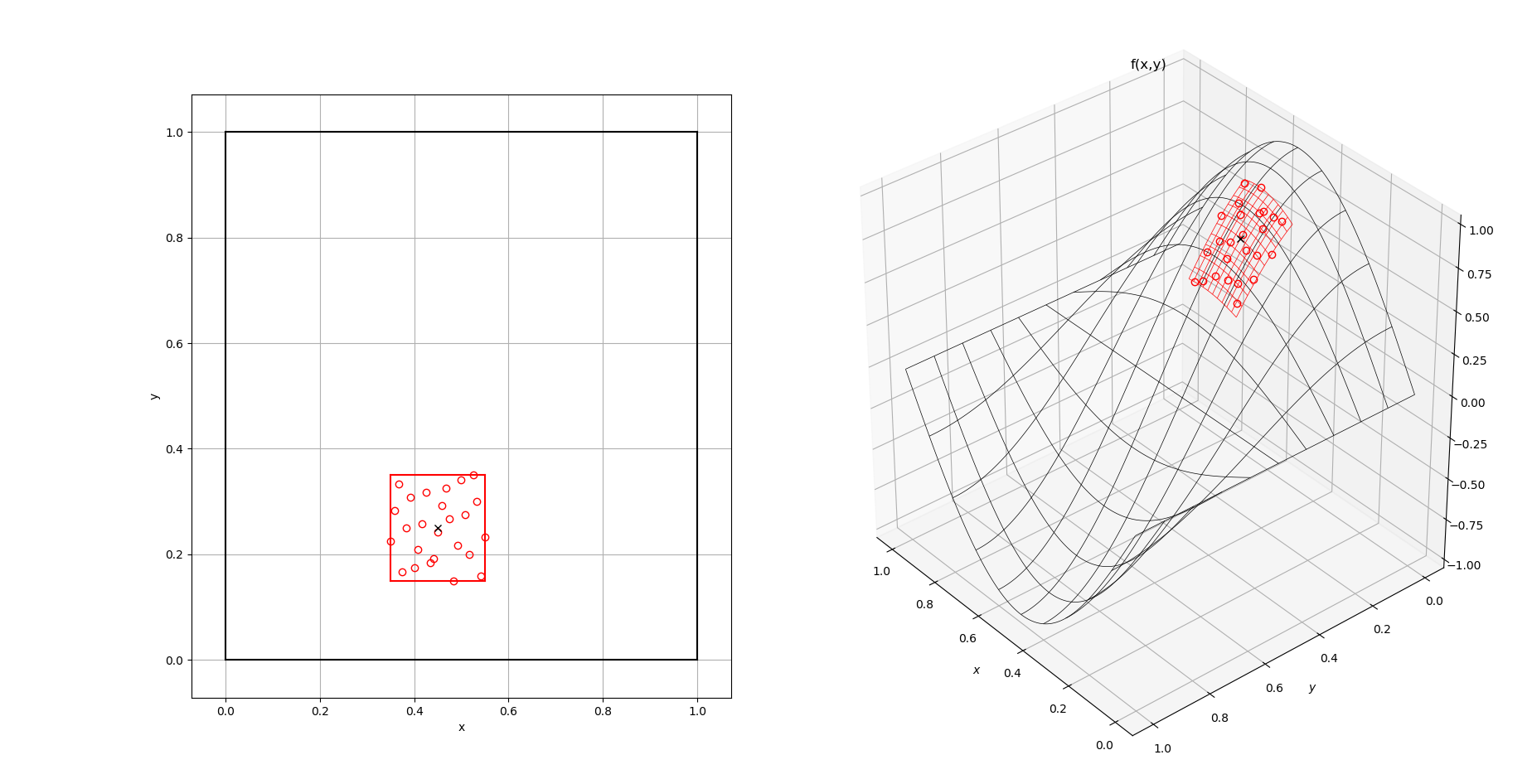
执行

细节：

numpy读取csv数据, output 格式为ndarray

us_file_path = "./data/US_video_data_numbers.csv"  # 数据存储路径
t_us = np.genfromtxt(us_file_path, delimiter=",")

scipy读取mat数据

import scipy.io as sio
data = sio.loadmat('train_data.mat');
data = data['data']

• 目前未解决：

/home/wjq/anaconda3/bin/python /home/wjq/文档/GitHub/MeshlessDerivatives/main.py
Traceback (most recent call last):
File “/home/wjq/文档/GitHub/MeshlessDerivatives/main.py”, line 183, in
main()
File “/home/wjq/文档/GitHub/MeshlessDerivatives/main.py”, line 177, in main
X,Y,Z = project_onto_regular_grid_2D(x, F, fit_order=2, nk=50)
File “/home/wjq/文档/GitHub/MeshlessDerivatives/main.py”, line 92, in project_onto_regular_grid_2D
solver.prepare( xi=x, xk=x[hoods] ) # generate problem matrices from the geometry of the point cloud
File “wlsqm/fitter/expert.pyx”, line 399, in wlsqm.fitter.expert.ExpertSolver.prepare
ValueError: Buffer and memoryview are not contiguous in the same dimension.

Process finished with exit code 1

¹. SIAM-Online dynamic mode decomposition for time-varying systems ↩

². Sherman, Adjustment of an inverse matrix corresponding to a change in one element of a given matrix. ↩

³. Hassan Arbabi, Spectral analysis of mixing in 2D high-Reynolds flows, JFM ↩

⁴. Study of dynamics in post-transient flows using Koopman mode decomposition-Physical review ↩

⁵. Geneative stochastic modeling of strongly nonlinear flows with non-Gaussian statistics ↩

⁶. Particles to Partial Differential Equations Parsimoniously ↩

⁷. Spectral analysis of mixing in 2D high-Reynolds flows” by H. Arbabi and I. Mezic ↩

⁸. Evolutionary Design Optimization with Nash Games and Hybridized Mesh/Meshless Methods in Computational Fluid Dynamics ↩

⁹: